
Section 7.3 Difference of two means using the \(t\)-distribution
¶Open Intro: Difference of two independent means
It is also useful to be able to compare two means for small samples. For instance, a teacher might like to test the notion that two versions of an exam were equally difficult. She could do so by randomly assigning each version to students. If she found that the average scores on the exams were so different that we cannot write it off as chance, then she may want to award extra points to students who took the more difficult exam.
In a medical context, we might investigate whether embryonic stem cells can improve heart pumping capacity in individuals who have suffered a heart attack. We could look for evidence of greater heart health in the stem cell group against a control group.
In this section we use the \(t\)-distribution for the difference in sample means. We will again drop the minimum sample size condition and instead impose a strong condition on the distribution of the data.
Subsection 7.3.1 Sampling distribution for the difference of two means
¶In this section we consider a difference in two population means, \(\mu_1 - \mu_2\text{,}\) under the condition that the data are not paired. The methods are similar in theory but different in the details. Just as with a single sample, we identify conditions to ensure a point estimate of the difference \(\bar{x}_1 - \bar{x}_2\) is nearly normal. Next we introduce a formula for the standard deviation of \(\bar{x}_1 - \bar{x}_2\text{,}\) which allows us to apply our general tools from Chapter 5.
We apply these methods to two examples: participants in the 2012 Cherry Blossom Run and newborn infants. This section is motivated by questions like “Is there convincing evidence that newborns from mothers who smoke have a different average birth weight than newborns from mothers who don't smoke?”
We start by looking at the population mean and standard deviation for the run times of men and women participants in the 2009 Cherry Blossom Run. Table 7.3.2 summarizes these values.
| men | women | |
| \(\mu\) | 87.65 | 102.13 |
| \(\sigma\) | 12.5 | 15.2 |
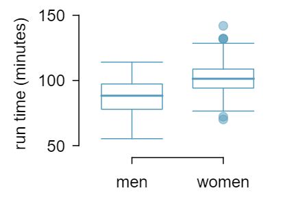
The two populations (men and women) are independent of one-another, so the data are not paired. 1 Probability theory guarantees that the difference of two independent normal random variables is also normal. Because each sample mean is nearly normal and observations in the samples are independent, we are assured the difference is also nearly normal. If we take two separate random samples of men and women from this race, what is the expected value for the difference in their average times? Not surprisingly, the expected value of \(\bar{x}_{w} - \bar{x}_{m}\) is \(\mu_1-\mu_2\text{.}\) We can quantify the variability in the point estimate, using the following formula for its standard deviation:
\begin{align*}
SD_{\bar{x}_{w} - \bar{x}_{m}}
\amp = \sqrt{\left(SD_{\bar{x}_{w}}\right)^2 +\left(SD_{\bar{x}_{m}}\right)^2 }\\
\amp = \sqrt{\left(\frac{\sigma_{\bar{x}_{w}}}{\sqrt{n_w}}\right)^2 + \left(\frac{\sigma_{\bar{x}_{m}}}{\sqrt{n_m}}\right)^2 }\\
\amp = \sqrt{\frac{\sigma_{w}^2}{n_{w}} + \frac{\sigma_{m}^2}{n_{m}}}
\end{align*}
Let's say we take a random sample of 55 women and a random sample of 45 men. Use the SD formula for the difference of two means to compute the SD for the difference in the average run time for males and females. 2 \(\sqrt{\frac{15.2^2}{55} + \frac{12.5^2}{45}} = 2.77\)
Distribution of a difference of sample means
The sample difference of two means, \(\bar{x}_1 - \bar{x}_2\text{,}\) is nearly normal with mean \(\mu_{1}-\mu_{2}\) and standard deviation
\begin{gather}
SD_{\bar{x}_{1} - \bar{x}_{2}} = \sqrt{\frac{\sigma_1^2}{n_1} + \frac{\sigma_2^2}{n_2}}\label{sdtwosample}\tag{7.3.1}
\end{gather}
when each sample mean is nearly normal and all observations are independent. Recall that each sample mean will be nearly normal if the population is normal or if the sample size is at least 30.
Subsection 7.3.2 Point estimates and standard errors for differences of means
In the example of two exam versions, the teacher would like to evaluate whether there is convincing evidence that the difference in average scores between the two exams is not due to chance.
It will be useful to extend the \(t\)-distribution method from Section 7.1 to apply to a difference of means:
\begin{gather*}
\bar{x}_1 - \bar{x}_2
\qquad \text{ as a point estimate for } \qquad
\mu_1 - \mu_2
\end{gather*}
First, we verify the small sample conditions (independence and nearly normal data) for each sample separately, then we verify that the samples are also independent. For instance, if the teacher believes students in her class are independent, the exam scores are nearly normal, and the students taking each version of the exam were independent, then we can use the \(t\)-distribution for inference on the point estimate \(\bar{x}_{1} - \bar{x}_{2}\text{.}\)
The formula for the standard error of \(\bar{x}_{1} - \bar{x}_{2}\text{,}\) introduced in Subsection 7.3.1, also applies to small samples:
\begin{gather}
SE_{\bar{x}_1 - \bar{x}_2}
= \sqrt{SE_{\bar{x}_1}^2 + SE_{\bar{x}_2}^2}
= \sqrt{\frac{s_1^2}{n_1} + \frac{s_2^2}{n_2}}\label{seOfDiffOfTwoMeansInTDistSection}\tag{7.3.2}
\end{gather}
Because we will use the \(t\)-distribution, we will need to identify the appropriate degrees of freedom. This can be done using a calculator or computer software. An alternative technique is to use the smaller of \(n_1 - 1\) and \(n_2 - 1\text{.}\) 3 This technique for degrees of freedom is conservative with respect to a Type 1 Error; it is more difficult to reject the null hypothesis using this \(df\) method.
Using the \(t\)-distribution for a difference in means
The \(t\)-distribution can be used for inference when working with the standardized difference of two means if (1) each sample meets the conditions for using the \(t\)-distribution and (2) the samples are independent. We estimate the standard error of the difference of two means using Equation (7.3.2).
Subsection 7.3.3 Hypothesis testing for the difference of two means
Summary statistics for each exam version are shown in Table 7.3.5. The teacher would like to evaluate whether this difference is so large that it provides convincing evidence that Version B was more difficult (on average) than Version A.
| Version | \(n\) | \(\bar{x}\) | \(s\) | min | max |
| A | 30 | 79.4 | 14 | 45 | 100 |
| B | 27 | 74.1 | 20 | 32 | 100 |
Guided Practice 7.3.6
Construct a two-sided hypothesis test to evaluate whether the observed difference in sample means, \(\bar{x}_A - \bar{x}_B=5.3\text{,}\) might be due to chance. 4 Because the teacher did not expect one exam to be more difficult prior to examining the test results, she should use a two-sided hypothesis test. \(H_0\text{:}\) the exams are equally difficult, on average. \(\mu_A - \mu_B = 0\text{.}\) \(H_A\text{:}\) one exam was more difficult than the other, on average. \(\mu_A - \mu_B \neq 0\text{.}\)
Guided Practice 7.3.7
To evaluate the hypotheses in Guided Practice 7.3.6 using the \(t\)-distribution, we must first verify assumptions. (a) Does it seem reasonable that the scores are independent within each group? (b) What about the normality condition for each group? (c) Do you think scores from the two groups would be independent of each other (i.e. the two samples are independent)? 5 (a) It is probably reasonable to conclude the scores are independent. (b) The summary statistics suggest the data are roughly symmetric about the mean, and it doesn't seem unreasonable to suggest the data might be normal. Note that since these samples are each nearing 30, moderate skew in the data would be acceptable. (c) It seems reasonable to suppose that the samples are independent since the exams were handed out randomly.
After verifying the conditions for each sample and confirming the samples are independent of each other, we are ready to conduct the test using the \(t\)-distribution. In this case, we are estimating the true difference in average test scores using the sample data, so the point estimate is \(\bar{x}_A - \bar{x}_B = 5.3\text{.}\) The standard error of the estimate can be calculated using Equation (7.3.2):
\begin{gather*}
SE = \sqrt{\frac{s_A^2}{n_A} + \frac{s_B^2}{n_B}} = \sqrt{\frac{14^2}{30} + \frac{20^2}{27}} = 4.62
\end{gather*}
Finally, we construct the test statistic:
\begin{gather*}
T = \frac{\text{ point estimate } - \text{ null value } }{SE} = \frac{(79.4-74.1) - 0}{4.62} = 1.15
\end{gather*}
If we have a calculator or computer handy, we can identify the degrees of freedom as 45.97. Otherwise we use the smaller of \(n_1-1\) and \(n_2-1\text{:}\) \(df=26\text{.}\)
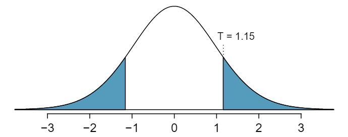
Guided Practice 7.3.9
Identify the p-value, shown in Figure 7.3.8. Use \(df=26\text{.}\) 6 We examine row \(df=26\) in the \(t\)-table. Because this value is smaller than the value in the left column, the p-value is larger than 0.200 (two tails!). Because the p-value is so large, we do not reject the null hypothesis. That is, the data do not convincingly show that one exam version is more difficult than the other, and the teacher should not be convinced that she should add points to the Version B exam scores.
In Guided Practice 7.3.9, we could have used \(df=45.97\text{.}\) However, this value is not listed in the table. In such cases, we use the next lower degrees of freedom (unless the computer also provides the p-value). For example, we could have used \(df=45\) but not \(df=46\text{.}\) As before, we provide a summary of the steps to perform when carrying out such a test.
Hypothesis test for the difference of two means
-
State the name of the test being used.
2-sample \(t\)-test.
-
Verify conditions.
2 independent random samples OR 2 randomly allocated treatments.
Both populations known to be normal OR \(n_1 \ge 30 \text{ and } n_2\ge 30\) OR graphs of both samples are approximately symmetric with no outliers, making the assumption that the populations are normal a reasonable one.
-
Write the hypotheses in plain language, then set them up in mathematical notation.
H\(_0: \mu_1 = \mu_2\) or \(\mu_1 - \mu_2 = 0\)
H\(_0: \mu_1 \ne \text{ or } \lt \text{ or } > \mu_2\)
Identify the significance level \(\alpha\text{.}\)
-
Calculate the test statistic and \(df\text{:}\) \(T = \frac{\text{ point estimate } - \text{ null value } }{\text{ SE of estimate } }\)
The point estimate is \(\bar{x}_1-\bar{x}_2\)
\(SE = \sqrt{\frac{s^2_1}{n_1}+\frac{s^2_2}{n_2}}\)
Find and record the \(df\) from a calculator.
Find the p-value and compare it to \(\alpha\) to determine whether to reject or not reject \(H_0\text{.}\)
Write the conclusion in the context of the question.
| \(n\) | \(\bar{x}\) | \(s\) | |||
| ESCs | 9 | 3.50 | 5.17 | ||
| control | 9 | -4.33 | 2.76 | ||
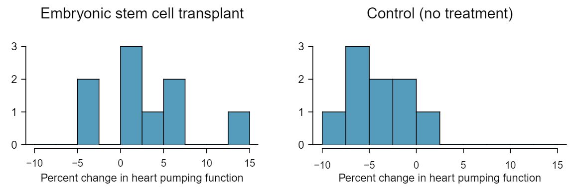
Example 7.3.12
Do embryonic stem cells (ESCs) help improve heart function following a heart attack? Table 7.3.10 contains summary statistics for an experiment to test ESCs in sheep that had a heart attack. Each of these sheep was randomly assigned to the ESC or control group, and the change in their hearts' pumping capacity was measured. A positive value generally corresponds to increased pumping capacity, which suggests a stronger recovery. The sample data is graphed in Figure 7.3.11. Use the given information and an appropriate an appopriate statistical test to answer the research question.
Solution
We will carry out a 2-sample \(t\)-test. The first condition is met because it is stated that there were two randomly allocated treatments. For the second condition, we must look at a graphs of the data. The data are very limited, so we can only check for obvious outliers in the raw data in Figure 7.3.11. Since the distributions are (very) roughly symmetric, we will assume the populations are approximately normal.
\(\mu_{esc} - \mu_{control} = 0\text{.}\) The stem cells do not improve heart pumping function.
\(\mu_{esc} - \mu_{control} \gt 0\text{.}\) The stem cells do improve heart pumping function.
Let \(\alpha=0.05\text{.}\) Now we compute the sample difference, the standard error for that point estimate, and the test statistic:
\begin{align*}
\amp \bar{x}_{esc} - \bar{x}_{control} = 7.83
\amp SE = \sqrt{\frac{5.17^2}{9} + \frac{2.76^2}{9}} = 1.95\\
\amp T = \frac{7.83 - 0}{1.95} = 4.01
\end{align*}
Using a calculator, \(df=12.2\) and p-value = \(8.4\text{x} 10^{-4}\text{.}\) The p-value is much less than 0.05, so we reject the null hypothesis. The data provide convincing evidence that embryonic stem cells improve the heart's pumping function in sheep that have suffered a heart attack.
Subsection 7.3.4 Confidence intervals for \(\mu_1-\mu_2\)
The results from the previous section provided evidence that ESCs actually help improve the pumping function of the heart. But how large is this improvement? To answer this question, we can use a confidence interval.
Confidence intervals take the form
\begin{gather*}
\text{ point estimate } \ \pm \text{ critical value } \times SE
\end{gather*}
Using the point estimate and the SE calculated in the previous section, we get the general form of a confidence interval for a difference in means, \(\mu_1-\mu_2\text{.}\)
\begin{gather*}
(\bar{x}_1-\bar{x}_2) \ \pm \ t^\star\sqrt{\frac{s_1^2}{n_1} + \frac{s_2^2}{n_2}}
\end{gather*}
Guided Practice 7.3.13
In Example 7.3.12, you found that the point estimate, \(\bar{x}_{esc} - \bar{x}_{control} = 7.83\text{,}\) has a standard error of 1.95. Using \(df=8\text{,}\) create a 99% confidence interval for the improvement due to ESCs. 7 We know the point estimate, 7.83, and the standard error, 1.95. We also verified the conditions for using the \(t\)-distribution in Example 7.3.12. Thus, we only need identify \(t^{\star}_8\) to create a 99% confidence interval: \(t^{\star}_{8} = 3.36\text{.}\) The 99% confidence interval for the improvement from ESCs is given by
\begin{align*}
\text{ point estimate } \ \amp \pm\ t^{\star}SE\\
7.83\ \amp \pm\ 3.36\times 1.95 df=8\\
(1.33 \amp \text{ , } 14.43)
\end{align*}
That is, we are 99% confident that the true improvement in heart pumping function is somewhere between 1.33% and 14.43%.
Constructing a confidence interval for the difference of two means
-
State the name of the CI being used.
2-sample \(t\)-interval.
-
Verify conditions.
2 independent random samples OR 2 randomly allocated treatments.
Both populations are known to be normal OR \(n_1 \text{ and } n_2\ge 30\) OR graphs of both samples are approximately symmetric with no outliers, i.e. the assumption that the populations are normal is reasonable.
-
Plug in the numbers and write the interval in the form
\begin{equation*} \text{ point estimate } \pm t^\star \times \text{ SE of estimate } \end{equation*}The point estimate is \(\bar{x}_1-\bar{x}_2\)
Find and record the \(df\) using a calculator
Find the critical value \(t^\star\) using the \(t\)-table at row = \(df\) (round down to nearest integer)
Use \(SE = \sqrt{\frac{s^2_1}{n_1}+\frac{s^2_2}{n_2}}\)
Evaluate the CI and write in the form ( \(\_\) , \(\_\) ).
Interpret the interval: ``We are [XX]% confident that the true difference in the mean of [...] is between [...] and [...]."
State the conclusion to the original question.
An instructor decided to run two slight variations of the same exam. Prior to passing out the exams, she shuffled the exams together to ensure each student received a random version. Summary statistics for how students performed on these two exams are shown in Table 7.3.14. Anticipating complaints from students who took Version B, she would like to evaluate whether the difference observed in the groups is so large that it provides convincing evidence that Version B was more difficult (on average) than Version A.
| Version | \(n\) | \(\bar{x}\) | \(s\) | min | max |
| A | 30 | 79.4 | 14 | 45 | 100 |
| B | 27 | 74.1 | 20 | 32 | 100 |
Example 7.3.15
Construct a 90% confidence interval for the difference in average scores. At this confidence level, is there evidence that one test was more difficult than the other?
Solution
We have two randomly allocated treatments (tests) and the scores for both groups do not show excessive skew, so we can assume that the population distributions are approximately normal. The point estimate is \(\bar{x}_A - \bar{x}_B = 5.3\text{.}\) The standard error of the estimate can be calculated as
\begin{gather*}
SE = \sqrt{\frac{14^2}{30} + \frac{20^2}{27}} = 4.62
\end{gather*}
A calculator gives the degrees of freedom as 45.97. The confidence interval is given by \(5.3\ \pm \ 1.684(4.62)\to (-2.5, 13.1)\text{.}\) Because the interval contains both positive and negative values the data do not convincingly show that one exam version is more difficult than the other, and the teacher should not be convinced that she should add points to the Version B exam scores.
Subsection 7.3.5 Calculator: the 2-sample \(t\)-test and \(t\)-interval
TI-83/84: 2-sample \(t\)-test
MISSINGVIDEOLINK Use STAT, TESTS, 2-SampTTest.
Choose
STAT.Right arrow to
TESTS.Choose
4:2-SampTTest.-
Choose
Dataif you have all the data orStatsif you have the means and standard deviations.If you choose
Data, letList1beL1or the list that contains sample 1 and letList2beL2or the list that contains sample 2 (don't forget to enter the data!). LetFreq1andFreq2be1.If you choose
Stats, enter the mean, SD, and sample size for sample 1 and for sample 2
Choose \(\ne\text{,}\) \(\lt\text{,}\) or \(\gt\) to correspond to H\(_A\text{.}\)
Let
PooledbeNO.Choose
Calculateand hitENTER, which returns:tt statistic Sx1SD of sample 1 pp-value Sx2SD of sample 2 dfdegrees of freedom n1size of sample 1 \(\bar{x}_1\) mean of sample 1 n2 size of sample 2 \(\bar{x}_2\) mean of sample 2
Casio fx-9750GII: 2-sample \(t\)-test
MISSINGVIDEOLINK
Navigate to
STAT(MENUbutton, then hit the2button or selectSTAT).If necessary, enter the data into a list.
Choose the
TESToption (F3button).Choose the
toption (F2button).Choose the
2-Soption (F2button).Choose either the
Varoption (F2) or enter the data in using theListoption.-
Specify the test details:
Specify the sidedness of the test using the
F1,F2, andF3keys.If using the
Varoption, enter the summary statistics for each group. If usingList, specify the lists and leaveFreqvalues at1.Choose whether to pool the data or not.
Hit the
EXEbutton, which returns\(\mu1\ \_\_\ \mu2\) alt. hypothesis \(\bar{x}1\text{,}\) \(\bar{x}2\) sample means tt statistic sx1,sx2sample standard deviations pp-value n1,n2sample sizes dfdegrees of freedom
TI-83/84: 2-sample \(t\)-int\(t\)val
MISSINGVIDEOLINK Use STAT, TESTS, 2-SampTInt.
Choose
STAT.Right arrow to
TESTS.Down arrow and choose
0:2-SampTTInt.-
Choose
Dataif you have all the data orStatsif you have the means and standard deviations.If you choose Data, let
List1beL1or the list that contains sample 1 and letList2beL2or the list that contains sample 2 (don't forget to enter the data!). LetFreq1andFreq2be1.If you choose
Stats, enter the mean, SD, and sample size for sample 1 and for sample 2.
Let
C-Levelbe the desired confidence level and letPooledbeNo.Choose
Calculateand hitENTER, which returns:(,)the confidence interval Sx1SD of sample 1 dfdegrees of freedom Sx2SD of sample 2 \(\bar{x}_1\) mean of sample 1 n1size of sample 1 \(\bar{x}_2\) mean of sample 2 n2size of sample 2
Casio fx-9750GII: 2-sample \(t\)-interval
MISSINGVIDEOLINK
Navigate to
STAT(MENUbutton, then hit the2button or selectSTAT).If necessary, enter the data into a list.
Choose the
INTRoption (F4button).Choose the
toption (F2button).Choose the
2-Soption (F2button).Choose either the
Varoption (F2) or enter the data in using theListoption.-
Specify the test details:
Confidence level of interest for
C-Level.If using the
Varoption, enter the summary statistics for each group. If usingList, specify the lists and leaveFreqvalues at1.Choose whether to pool the data or not.
Hit the
EXEbutton, which returnsLeft,Rightends of the confidence interval dfdegrees of freedom \(\bar{x}1\text{,}\) \(\bar{x}2\) sample means sx1,sx2sample standard deviations n1,n2sample sizes
Guided Practice 7.3.16
Use the data from the ESC experiment shown in Table 7.3.17 and a calculator to find the appropriate degrees of freedom and construct a 90% confidence interval. 8 The interval is \((4.3543, 11.307)\) with \(df=12.2\text{.}\)
| \(n\) | \(\bar{x}\) | \(s\) | |||
| ESCs | 9 | 3.50 | 5.17 | ||
| control | 9 | -4.33 | 2.76 | ||
Guided Practice 7.3.18
Use the data from the ESC example and a calculator to find an appropriate statistic, degrees of freedom, and p-value for a two-sided hypothesis test. 9 \(T=4.008\text{,}\) \(df=12.2\text{,}\) and p-value\(=0.00168\text{.}\)