Advanced High School Statistics: First Edition

Subsection 1.4.1 Observational studies

Generally, data in observational studies are collected only by monitoring what occurs, while experiments require the primary explanatory variable in a study be assigned for each subject by the researchers.

Making causal conclusions based on experiments is often reasonable. However, making the same causal conclusions based on observational data is treacherous and is not recommended. Observational studies are generally only sufficient to show associations.

Some previous research tells us that using sunscreen actually reduces skin cancer risk, so maybe there is another variable that can explain this hypothetical association between sunscreen usage and skin cancer. One important piece of information that is absent is sun exposure. Sun exposure is what is called a confounding variable (also called a lurking variable, confounding factor, or a confounder).

Sun exposure is a confounding factor because it is associated with both the use of sunscreen and the development of skin cancer. People who are out in the sun all day are more likely to use sunscreen, and people who are out in the sun all day are more likely to get skin cancer. Research shows us the development of skin cancer is due to the sun exposure. The variables of sunscreen usage and sun exposure are confounded, and without this research, we would have no way of knowing which one was the true cause of skin cancer.

While one method to justify making causal conclusions from observational studies is to exhaust the search for confounding variables, there is no guarantee that all confounding variables can be examined or measured.

In the same way, the county data set is an observational study with confounding variables, and its data cannot be used to make causal conclusions.

Observational studies come in two forms: prospective and retrospective studies. A prospective study identifies individuals and collects information as events unfold. For instance, medical researchers may identify and follow a group of similar individuals over many years to assess the possible influences of behavior on cancer risk. One example of such a study is The Nurses' Health Study, started in 1976 and expanded in 1989.⁴www.channing.harvard.edu/nhs This prospective study recruits registered nurses and then collects data from them using questionnaires. Retrospective studies collect data after events have taken place, e.g. researchers may review past events in medical records. Some data sets, such as county, may contain both prospectively- and retrospectively-collected variables. Local governments prospectively collect some variables as events unfolded (e.g. retails sales) while the federal government retrospectively collected others during the 2010 census (e.g. county population counts).

Subsection 1.4.2 Sampling from a population

We might try to estimate the time to graduation for Duke undergraduates in the last 5 years by collecting a sample of students. All graduates in the last 5 years represent the population, and graduates who are selected for review are collectively called the sample. In general, we always seek to randomly select a sample from a population. The most basic type of random selection is equivalent to how raffles are conducted. For example, in selecting graduates, we could write each graduate's name on a raffle ticket and draw 100 tickets. The selected names would represent a random sample of 100 graduates.

Why pick a sample randomly? Why not just pick a sample by hand? Consider the following scenario.

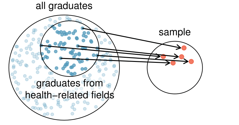
If the student majoring in nutrition picked a disproportionate number of graduates from health-related fields, this would introduce selection bias into the sample. Selection bias occurs when some individuals of the population are inherently more likely to be included in the sample than others. In the example, this bias creates a problem because a degree in health-related fields might take more or less time to complete than a degree in other fields. Suppose that it takes longer. Since graduates from health-related fields would be more likely to be in the sample, the selection bias would cause her to overestimate the parameter.

Sampling randomly resolves the problem of selection bias. The most basic random sample is called a simple random sample, which is equivalent to using a raffle to select cases. This means that each case in the population has an equal chance of being included and there is no implied connection between the cases in the sample.

A common downfall is a convenience sample, where individuals who are easily accessible are more likely to be included in the sample. For instance, if a political survey is done by stopping people walking in the Bronx, this will not represent all of New York City. It is often difficult to discern what sub-population a convenience sample represents.

Similarly, a volunteer sample is one in which people's responses are solicited and those who choose to participate, respond. This is a problem because those who choose to participate may tend to have different opinions than the rest of the population, resulting in a biased sample.

The act of taking a random sample helps minimize bias; however, bias can crop up in other ways. Even when people are picked at random, e.g. for surveys, caution must be exercised if the non-response is high. For instance, if only 30% of the people randomly sampled for a survey actually respond, then it is unclear whether the results are representative of the entire population. This non-response bias can skew results.

Even if a sample has no selection bias and no non-response bias, there is an additional type of bias that often crops up and undermines the validity of results, known as response bias. Response bias refers to a broad range of factors that influence how a person responds, such as question wording, question order, and influence of the interviewer. This type of bias can be present even when we collect data from an entire population in what is called a census. Because response bias is often subtle, one must pay careful attention to how questions were asked when attempting to draw conclusions from the data.

When there is no bias in a sample, increasing the sample size tends to increase the precision and reliability of the estimate. When a sample is biased, it may be impossible to decipher helpful information from the data, even if the sample is very large.

Subsection 1.4.3 Simple, systematic, stratified, cluster, and multistage sampling

Almost all statistical methods for observational data rely on a sample being random and unbiased. When a sample is collected in a biased way, these statistical methods will not generally produce reliable information about the population.

The idea of a simple random sample was introduced in the last section. Here we provide a more technical treatment of this method and introduce four new random sampling methods: systematic, stratified, cluster, and multistage.⁷Systematic and Multistage sampling are not part of the AP syllabus. Figure 1.4.13 provides a graphical representation of simple versus systematic sampling while Figure 1.4.15 provides a graphical representation of stratified, cluster, and multistage sampling.

Simple random sampling is probably the most intuitive form of random sampling. Consider the salaries of Major League Baseball (MLB) players, where each player is a member of one of the league's 30 teams. For the 2010 season, N, the population size or total number of players, is 828. To take a simple random sample of n = 120 of these baseball players and their salaries, we could number each player from 1 to 828. Then we could randomly select 120 numbers between 1 and 828 (without replacement) using a random number generator or random digit table. The players with the selected numbers would comprise our sample.

Two properties are always true in a simple random sample:

1. Each case in the population has an equal chance of being included in the sample.

2. Each group of n cases has an equal chance of making up the sample.

The statistical methods in this book focus on data collected using simple random sampling. Note that Property 2 — that each group of n cases has an equal chance making up the sample — is not true for the reidxing four sampling techniques. As you read each one, consider why.

Though less common than simple random sampling, systematic sampling is sometimes used when there exists a convenient list of all of the individuals of the population. Suppose we have a roster with the names of all the MLB players from the 2010 season. To take a systematic random sample, number them from 1 to 828. Select one random number between 1 and 828 and let that player be the first individual in the sample. Then, depending on the desired sample size, select every 10th number or 20th number, for example, to arrive at the sample.⁸If we want a sample of size n = 138, it would make sense to select every 6th player since \(828/138 = 6\text{.}\) Suppose we randomly select the number 810. Then player 810, 816, 822, 828, 6, 12, \(\cdots\) , 798, and 804 would make up the sample. If there are no patterns in the salaries based on the numbering then this could be a reasonable method.

Sometimes there is a variable that is known to be associated with the quantity we want to estimate. In this case, a stratified random sample might be selected. Stratified sampling is a divide-and-conquer sampling strategy. The population is divided into groups called strata. The strata are chosen so that similar cases are grouped together and a sampling method, usually simple random sampling, is employed to select a certain number or a certain proportion of the whole within each stratum. In the baseball salary example, the 30 teams could represent the strata; some teams have a lot more money (we're looking at you, Yankees).

Stratified sampling is inherently different than simple random sampling. For example, the stratified sampling approach described would make it impossible for the entire Yankees team to be included in the sample.

Next, let's consider a sampling technique that randomly selects groups of people. Cluster sampling is much like simple random sampling, but instead of randomly selecting individuals, we randomly select groups or clusters. Unlike stratified sampling, cluster sampling is most helpful when there is a lot of case-to-case variability within a cluster but the clusters themselves don't look very different from one another. That is, we expect strata to be self-similar (homogeneous), while we expect clusters to be diverse (heterogeneous).

Sometimes cluster sampling can be a more economical random sampling technique than the alternatives. For example, if neighborhoods represented clusters, this sampling method works best when each neighborhood is very diverse. Because each neighborhood itself encompasses diversity, a cluster sample can reduce the time and cost associated with data collection, because the interviewer would need only go to some of the neighborhoods rather than to all parts of a city, in order to collect a useful sample.

Multistage sampling, also called multistage cluster sampling, is a two (or more) step strategy. The first step is to take a cluster sample, as described above. Then, instead of including all of the individuals in these clusters in our sample, a second sampling method, usually simple random sampling, is employed within each of the selected clusters. In the neighborhood example, we could first randomly select some number of neighborhoods and then take a simple random sample from just those selected neighborhoods. As seen in Figure 1.4.15, stratified sampling requires observations to be sampled from every stratum. Multistage sampling selects observations only from those clusters that were randomly selected in the first step.

It is also possible to have more than two steps in multistage sampling. Each cluster may be naturally divided into subclusters. For example, each neighborhood could be divided into streets. To take a three-stage sample, we could first select some number of clusters (neighborhoods), and then, within the selected clusters, select some number of subclusters (streets). Finally, we could select some number of individuals from each of the selected streets.