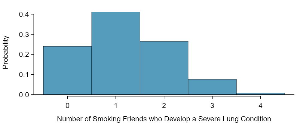
As in Example 4.4.6, we leave it to the reader to show that the binomial model is reasonable for this context. However, we will verify that both \(np\) and \(n(1-p)\) are at least 10 so we can apply the normal model:
\begin{align*}
np\amp =400(0.20)=80\ge 10\\
n(1-p)\amp =400(0.8)=320\ge 10
\end{align*}
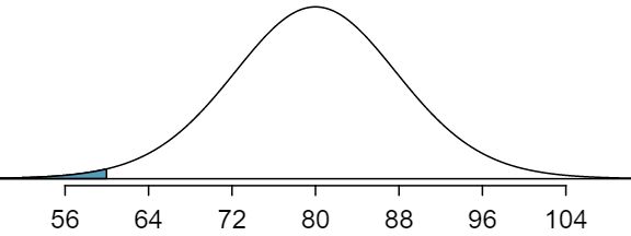
With these conditions checked, we may use the normal approximation in place of the binomial distribution with the following mean and standard deviation:
\begin{align*}
\mu \amp = np = 400(0.2)=80\\
\sigma \amp = \sqrt{np(1-p)} = \sqrt{400(0.2)(0.8)}= 8
\end{align*}
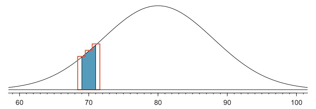
We want to find the probability of observing 60 or fewer smokers using this model. We know that this probability will be small because 60 is more than 2 standard deviations below the mean:
Next, we compute the Z-score as \(Z=\frac{60 - 80}{8} = -2.5\) to find the shaded area in the picture: \(P(Z \lt -2.5) = 0.0062\text{.}\) This probability of 0.0062 using the normal approximation is remarkably close to the true probability of 0.0061 from the binomial distribution!