
Section 5.2 Confidence intervals
¶OpenIntro: Confidence Intervals
A point estimate provides a single plausible value for a parameter. However, a point estimate is rarely perfect; usually there is some error in the estimate. In addition to supplying a point estimate of a parameter, a next logical step would be to provide a plausible range of values for the parameter.
Subsection 5.2.1 Capturing the population parameter
A plausible range of values for the population parameter is called a confidence interval. Using only a point estimate is like fishing in a murky lake with a spear, and using a confidence interval is like fishing with a net. We can throw a spear where we saw a fish, but we will probably miss. On the other hand, if we toss a net in that area, we have a good chance of catching the fish.
If we report a point estimate, we probably will not hit the exact population parameter. On the other hand, if we report a range of plausible values — a confidence interval — we have a good shot at capturing the parameter.
If we want to be very confident we capture the population parameter, should we use a wider interval or a smaller interval? 1 If we want to be more confident we will capture the fish, we might use a wider net. Likewise, we use a wider confidence interval if we want to be more confident that we capture the parameter.
Subsection 5.2.2 Constructing a 95% confidence interval
A point estimate is our best guess for the value of the parameter, so it makes sense to build the confidence interval around that value. The standard error, which is a measure of the uncertainty associated with the point estimate, provides a guide for how large we should make the confidence interval.
Constructing a 95% confidence interval
When the sampling distribution of a point estimate can reasonably be modeled as normal, the point estimate we observe will be within 1.96 standard errors of the true value of interest about 95% of the time. Thus, a 95% confidence interval for such a point estimate can be constructed:
\begin{gather}
\text{ point estimate } \ \pm\ 1.96 \times SE\label{basic_ci_formula}\tag{5.2.1}
\end{gather}
We can be 95% confident this interval captures the true value.
Guided Practice 5.2.3
Compute the area between -1.96 and 1.96 for a normal distribution with mean 0 and standard deviation 1. 2 We will leave it to you to draw a picture. The Z-scores are \(Z_{left} = -1.96\) and \(Z_{right} = 1.96\text{.}\) The area between these two Z-scores is \(0.9500\text{.}\) This is where “1.96” comes from in the 95% confidence interval formula.
Example 5.2.4
The point estimate from the smoking example was 15%. In the next chapters we will determine when we can apply a normal model to a point estimate. For now, assume that the normal model is reasonable. The standard error for this point estimate was calculated to be \(SE = 0.04\text{.}\) Construct a 95% confidence interval.
Solution
\begin{align*}
\text{ point estimate } \ \amp \pm \ 1.96\times SE\\
0.15\ \amp \pm \ 1.96\times 0.04\\
(0.0716\amp \text{ , } 0.2284)
\end{align*}
We are 95% confident that the true percent of smokers in this population is between 7.16% and 22.84%.
Example 5.2.5
Based on the confidence interval above, is there evidence that a smaller proportion smoke in this county than in the state as a whole? The proportion that smoke in the state is known to be 0.20.
Solution
While the point estimate of 0.15 is lower than 0.20, this deviation is likely due to random chance. Because the confidence interval includes the value 0.20, 0.20 is a reasonable value for the proportion of smokers in the county. Therefore, based on this confidence interval, we do not have evidence that a smaller proportion smoke in the county than in the state.
In Section 1.1 we encountered an experiment that examined whether implanting a stent in the brain of a patient at risk for a stroke helps reduce the risk of a stroke. The results from the first 30 days of this study, which included 451 patients, are summarized in Table 5.2.6. These results are surprising! The point estimate suggests that patients who received stents may have a higher risk of stroke: \(p_{trmt} - p_{ctrl} = 0.090\text{.}\)
| stroke | no event | Total | |
| treatment | 33 | 191 | 224 |
| control | 13 | 214 | 227 |
| Total | 46 | 405 | 451 |
Example 5.2.7
Consider the stent study and results. The conditions necessary to ensure the point estimate \(p_{trmt} - p_{ctrl} = 0.090\) is nearly normal have been verified for you, and the estimate's standard error is \(SE = 0.028\text{.}\) Construct a 95% confidence interval for the change in 30-day stroke rates from usage of the stent.
Solution
The conditions for applying the normal model have already been verified, so we can proceed to the construction of the confidence interval:
\begin{align*}
\text{ point estimate } \ \amp \pm \ 1.96\times SE\\
0.090\ \amp \pm \ 1.96 \times 0.028\\
(0.035\amp \text{ , } 0.145)
\end{align*}
We are 95% confident that implanting a stent in a stroke patient's brain. Since the entire interval is greater than 0, it means the data provide statistically significant evidence that the stent used in the study increases the risk of stroke, contrary to what researchers had expected before this study was published!
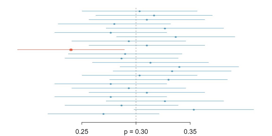
We can be 95% confident that a 95% confidence interval contains the true population parameter. However, confidence intervals are imperfect. About 1-in-20 (5%) properly constructed 95% confidence intervals will fail to capture the parameter of interest. Figure 5.2.8 shows 25 confidence intervals for a proportion that were constructed from simulations where the true proportion was \(p = 0.3\text{.}\) However, 1 of these 25 confidence intervals happened not to include the true value.
Guided Practice 5.2.9
In Figure 5.2.8, one interval does not contain the true proportion, \(p = 0.3\text{.}\) Does this imply that there was a problem with the simulations? 3 No. Just as some observations occur more than 1.96 standard deviations from the mean, some point estimates will be more than 1.96 standard errors from the parameter. A confidence interval only provides a plausible range of values for a parameter. While we might say other values are implausible based on the data, this does not mean they are impossible.
Subsection 5.2.3 Changing the confidence level
¶Suppose we want to consider confidence intervals where the confidence level is somewhat higher than 95%: perhaps we would like a confidence level of 99%.
Example 5.2.10
Would a 99% confidence interval be wider or narrower than a 95% confidence interval?
Solution
Using a previous analogy: if we want to be more confident that we will catch a fish, we should use a wider net, not a smaller one. To be 99% confidence of capturing the true value, we must use a wider interval. On the other hand, if we want an interval with lower confidence, such as 90%, we would use a narrower interval.
The 95% confidence interval structure provides guidance in how to make intervals with new confidence levels. Below is a general 95% confidence interval for a point estimate that comes from a nearly normal distribution:
\begin{gather}
\text{ point estimate } \ \pm\ 1.96\times SE\label{nine_five_ci}\tag{5.2.2}
\end{gather}
There are three components to this interval: the point estimate, “1.96”, and the standard error. The choice of \(1.96\times SE\) was based on capturing 95% of the distribution since the estimate is within 1.96 standard deviations of the true value about 95% of the time. The choice of 1.96 corresponds to a 95% confidence level.
Guided Practice 5.2.11
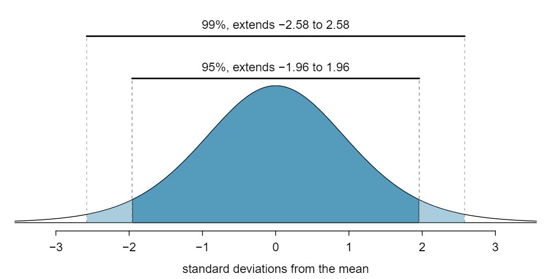
If \(X\) is a normally distributed random variable, how often will \(X\) be within 2.58 standard deviations of the mean? 4 This is equivalent to asking how often the Z-score will be larger than -2.58 but less than 2.58. (For a picture, see Figure 5.2.12.) There is \(\approx\) 0.99 probability that the unobserved random variable \(X\) will be within 2.58 standard deviations of the mean.
To create a 99% confidence interval, change 1.96 in the 95% confidence interval formula to be \(2.58\text{.}\) Guided Practice 5.2.11 highlights that 99% of the time a normal random variable will be within 2.58 standard deviations of its mean. This approach — using the Z-scores in the normal model to compute confidence levels — is appropriate when the point estimate is associated with a normal distribution and we can properly compute the standard error. Thus, the formula for a 99% confidence interval is
\begin{gather}
\text{ point estimate } \ \pm\ 2.58\times SE\label{nine_nine_ci}\tag{5.2.3}
\end{gather}
Figure 5.2.12 provides a picture of how to identify \(z^{\star}\) based on a confidence level.
Guided Practice 5.2.13
Create a 99% confidence interval for the impact of the stent on the risk of stroke using the data from Example 5.2.7. The point estimate is 0.090, and the standard error is \(SE = 0.028\text{.}\) It has been verified for you that the point estimate can reasonably be modeled by a normal distribution. 5 Since the necessary conditions for applying the normal model have already been checked for us, we can go straight to the construction of the confidence interval:
\begin{gather*}
\text{ point estimate } \ \pm\ 2.58 \times SE \rightarrow (0.018, 0.162)\text{.}
\end{gather*}
We are 99% confident that implanting a stent in the brain of a patient who is at risk of stroke increases the risk of stroke within 30 days by a rate of 0.018 to 0.162 (assuming the patients are representative of the population).
Confidence interval for any confidence level
If the point estimate follows the normal model with standard error \(SE\text{,}\) then a confidence interval for the population parameter is
\begin{gather*}
\text{ point estimate } \ \pm\ z^{\star} \times SE
\end{gather*}
where \(z^{\star}\) depends on the confidence level selected.
Finding the value of \(z^{\star}\) that corresponds to a particular confidence level is most easily accomplished by using a new table, called the \(t\)-table. For now, what is noteworthy about this table is that the bottom row corresponds to confidence levels. The numbers inside the table are the critical values, but which row should we use? Later in this book, we will see that a t curve with infinite degrees of freedom corresponds to the normal curve. For this reason, when finding using the \(t\)-table to find the appropriate \(z^{\star}\text{,}\) always use row \(\infty\text{.}\)
| one tail | 0.100 | 0.050 | 0.025 | 0.010 | 0.005 | |
| df | 1 | 3.078 | 6.314 | 12.71 | 31.82 | 63.66 |
| 2 | 1.886 | 2.920 | 4.303 | 6.965 | 9.925 | |
| 3 | 1.638 | 2.353 | 3.182 | 4.541 | 5.841 | |
| \(\vdots\) | \(\vdots\) | \(\vdots\) | \(\vdots\) | \(\vdots\) | ||
| 1000 | 1.282 | 1.646 | 1.962 | 2.330 | 2.581 | |
| \(\infty\) | 1.282 | 1.645 | 1.960 | 2.326 | 2.576 | |
| Confidence level C | 80% | 90% | 95% | 98% | 99% | |
TIP: Finding \(z^{\star}\) for a particular confidence level
We select \(z^{\star}\) so that the area between -\(z^{\star}\) and \(z^{\star}\) in the normal model corresponds to the confidence level. Use the \(t\)-table at row \(\infty\) to find the critical value \(z^{\star}\text{.}\)
Guided Practice 5.2.15
In Example 5.2.7 we found that implanting a stent in the brain of a patient at risk for a stroke increased the risk of a stroke. The study estimated a 9% increase in the number of patients who had a stroke, and the standard error of this estimate was about \(SE = 2.8\%\) or 0.028. Compute a 90% confidence interval for the effect. Note: the conditions for normality had earlier been confirmed for us. 6 We must find \(z^{\star}\) such that 90% of the distribution falls between -\(z^{\star}\) and \(z^{\star}\) in the standard normal model. Using the \(t\)-table with a confidence level of 90% at row \(\infty\) gives 1.645. Thus \(z^{\star}=1.645\text{.}\) The 90% confidence interval can then be computed as
\begin{align*}
\text{ point estimate } \ \amp \pm\ z^{\star}\times SE\\
0.09 \ \amp \pm \ 1.645\times 0.028\\
(0.044\amp \text{ , } 0.136)
\end{align*}
That is, we are 90% confident that implanting a stent in a stroke patient's brain increased the risk of stroke within 30 days by 4.4% to 13.6%.
The normal approximation is crucial to the precision of these confidence intervals. The next two chapters provides detailed discussions about when the normal model can safely be applied to a variety of situations. When the normal model is not a good fit, we will use alternate distributions that better characterize the sampling distribution.
Subsection 5.2.4 Margin of error
The confidence intervals we have encountered thus far have taken the form
\begin{gather*}
\text{ point estimate } \ \pm \ z^*\times SE
\end{gather*}
Confidence intervals are also often reported as
\begin{gather*}
\text{ point estimate } \ \pm \ \text{ margin of error }
\end{gather*}
For example, instead of reporting an interval as \(0.09 \ \pm \ 1.645\times 0.028\) or \((0.044, 0.136)\text{,}\) it could be reported as \(0.09 \ \pm \ 0.046\text{.}\)
The margin of error is the distance between the point estimate and the lower or upper bound of a confidence interval.
Margin of error
A confidence interval can be written as point estimate \(\pm\) margin of error. For a confidence interval for a proportion, the margin of error is \(z^{\star}\times SE\text{.}\)
Guided Practice 5.2.16
To have a smaller margin or error, should one use a larger sample or a smaller sample? 7 Intuitively, a larger sample should tend to yield less error. We can also note that \(n\text{,}\) the sample size is in the denominator of the SE formula, so a \(n\) goes up, the SE and thus the margin of error go down.
Guided Practice 5.2.17
What is the margin of error for the confidence interval: (0.035, 0.145)? 8 Because we both add and subtract the margin of error to get the confidence interval, the margin of error is half of the width of the interval. \((0.145 - 0.035)/2=0.055\text{.}\)
Subsection 5.2.5 Interpreting confidence intervals
¶A careful eye might have observed the somewhat awkward language used to describe confidence intervals. Correct interpretation:
We are [XX]% confident that the population parameter is between...
Incorrect language might try to describe the confidence interval as capturing the population parameter with a certain probability. 9 To see that this interpretation is incorrect, imagine taking two random samples and constructing two 95% confidence intervals for an unknown proportion. If these intervals are disjoint, can we say that there is a 95%+95%=190% chance that the first or the second interval captures the true value? This is one of the most common errors: while it might be useful to think of it as a probability, the confidence level only quantifies how plausible it is that the parameter is in the interval.
As we saw in Figure 5.2.8, the 95% confidence interval method has a 95% probability of producing an interval that will contain the population parameter. A correct interpretation of the confidence level is that such intervals will contain the population parameter that percent of the time. However, each individual interval either does or does not contain the population parameter. A correct interpretation of an individual confidence interval cannot involve the vocabulary of probability.
Another especially important consideration of confidence intervals is that they only try to capture the population parameter. Our intervals say nothing about the confidence of capturing individual observations, a proportion of the observations, or about capturing point estimates. Confidence intervals only attempt to capture population parameters.
Subsection 5.2.6 Using confidence intervals: a stepwise approach
Follow these six steps when carrying out any confidence interval problem.
Steps for using confidence intervals (AP exam tip)
The AP exam is scored in a standardized way, so to ensure full points for a problem, make sure to complete each of the following steps.
State the name of the CI being used.
Verify conditions to ensure the standard error estimate is reasonable and the point estimate is unbiased and follows the expected distribution, often a normal distribution.
-
Plug in the numbers and write the interval in the form
\begin{gather*} \text{ point estimate } \pm \text{ critical value } \times \text{ SE of estimate } \end{gather*}So far, the critical value has taken the form \(z^\star\text{.}\)
Evaluate the CI and write in the form (___,___).
Interpret the interval: “We are [XX]% confident that the true [describe the parameter in context] falls between [identify the upper and lower endpoints of the calculated interval].”
State your conclusion to the original question. (Sometimes, as in the case of the examples in this section, no conclusion is necessary.)