
Degrees of freedom (df)
The degrees of freedom describe the shape of the \(t\)-distribution. The larger the degrees of freedom, the more closely the distribution approximates the normal model.
When certain conditions are satisfied, the sampling distribution associated with a sample mean or difference of two sample means is nearly normal. However, this becomes more complex when the sample size is small, where small here typically means a sample size smaller than 30 observations. For this reason, we'll use a new distribution called the \(t\)-distribution that will often work for both small and large samples of numerical data.
We have seen in Section 4.2 that the distribution of a sample mean is normal if the population is normal or if the sample size is at least 30. In these problems, we used the population mean and population standard deviation to find a Z-score. However, in the case of inference, the parameters will be unknown. In rare circumstances we may know the standard deviation of a population, even though we do not know its mean. For example, in some industrial process, the mean may be known to shift over time, while the standard deviation of the process remains the same. In these cases, we can use the normal model as the basis for our inference procedures. We use \(\bar{x}\) as our point estimate for \(\mu\) and the SD formula calculated in Section 4.2: \(SD =\frac{\sigma}{\sqrt{n}}\text{.}\)
What happens if we do not know the population standard deviation \(\sigma\text{,}\) as is usually the case? The best we can do is use the sample standard deviation, denoted by \(s\text{,}\) to estimate the population standard deviation.
However, when we do this we run into a problem: when carrying out our inference procedures we will be trying to estimate two quantities: both the mean and the standard deviation. Looking at the SD and SE formulas, we can make some important observations that will give us a hint as to what will happen when we use \(s\) instead of \(\sigma\text{.}\)
For a given population, \(\sigma\) is a fixed number and does not vary.
\(s\text{,}\) the standard deviation of a sample, will vary from one sample to the next and will not be exactly equal to \(\sigma\text{.}\)
The larger the sample size \(n\text{,}\) the better the estimate \(s\) will tend to be for \(\sigma\text{.}\)
For this reason, the normal model still works well when the sample size is larger than about 30. For smaller sample sizes, we run into a problem: our estimate of \(s\text{,}\) which is used to compute the standard error, isn't as reliable and tends to add more variability to our estimate of the mean. It is this extra variability that leads us to a new distribution: the \(t\)-distribution.
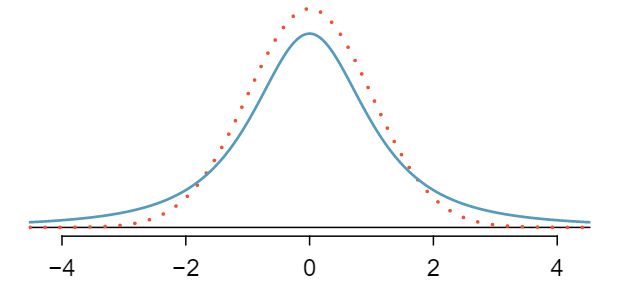
When we use the sample standard deviation \(s\) in place of the population standard deviation \(\sigma\) to standardize the sample mean, we get an entirely new distribution - one that is similar to the normal distribution, but has greater spread. This distribution is known as the \(t\)-distribution. A \(t\)-distribution, shown as a solid line in Figure 7.1.3, has a bell shape. However, its tails are thicker than the normal model's. This means observations are more likely to fall beyond two standard deviations from the mean than under the normal distribution. 1 The standard deviation of the \(t\)-distribution is actually a little more than 1. However, it is useful to always think of the \(t\)-distribution as having a standard deviation of 1 in all of our applications. These extra thick tails are exactly the correction we need to resolve the problem of a poorly estimated standard deviation.
The \(t\)-distribution, always centered at zero, has a single parameter: degrees of freedom. The degrees of freedom (df) describe the precise form of the bell-shaped \(t\)-distribution. Several \(t\)-distributions are shown in Figure 7.1.4. When there are more degrees of freedom, the \(t\)-distribution looks very much like the standard normal distribution.
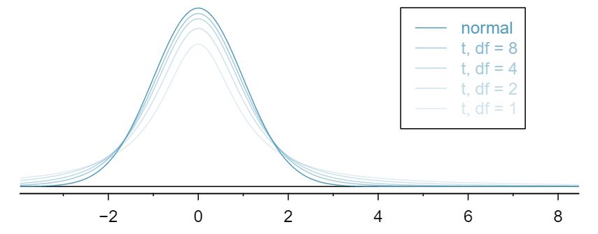
The degrees of freedom describe the shape of the \(t\)-distribution. The larger the degrees of freedom, the more closely the distribution approximates the normal model.
When the degrees of freedom is about 30 or more, the \(t\)-distribution is nearly indistinguishable from the normal distribution. In Subsection 7.1.3, we relate degrees of freedom to sample size.
We will find it very useful to become familiar with the \(t\)-distribution, because it plays a very similar role to the normal distribution during inference for numerical data. We use a \(t\)-table, partially shown in Table 7.1.5, in place of the normal probability table for numerical data when the population standard deviation is unknown, especially when the sample size is small. A larger table is presented in Appendix C.
| one tail | 0.100 | 0.050 | 0.025 | 0.010 | 0.005 | |
| \(df\) | 1 | 3.078 | 6.314 | 12.71 | 31.82 | 63.66 |
| 2 | 1.886 | 2.920 | 4.303 | 6.965 | 9.925 | |
| 3 | 1.638 | 2.353 | 3.182 | 4.541 | 5.841 | |
| \(\vdots\) | \(\vdots\) | \(\vdots\) | \(\vdots\) | \(\vdots\) | ||
| 17 | 1.333 | 1.740 | 2.110 | 2.567 | 2.898 | |
| 18 | 1.330 | 1.734 | 2.101 | 2.552 | 2.878 | |
| 19 | 1.328 | 1.729 | 2.093 | 2.539 | 2.861 | |
| 20 | 1.325 | 1.725 | 2.086 | 2.528 | 2.845 | |
| \(\vdots\) | \(\vdots\) | \(\vdots\) | \(\vdots\) | \(\vdots\) | ||
| 1000 | 1.282 | 1.646 | 1.962 | 2.330 | 2.581 | |
| \(\infty\) | 1.282 | 1.645 | 1.960 | 2.326 | 2.576 | |
| Confidence level C | 80% | 90% | 95% | 98% | 99% | |
Each row in the \(t\)-table represents a \(t\)-distribution with different degrees of freedom. The columns correspond to tail probabilities. For instance, if we know we are working with the \(t\)-distribution with \(df=18\text{,}\) we can examine row 18, which is highlighted in Table 7.1.5. If we want the value in this row that identifies the cutoff for an upper tail of 10%, we can look in the column where one tail is 0.100. This cutoff is 1.33. If we had wanted the cutoff for the lower 10%, we would use -1.33. Just like the normal distribution, all \(t\)-distributions are symmetric.
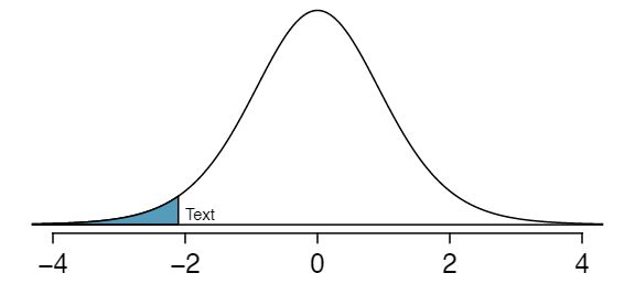
What proportion of the \(t\)-distribution with 18 degrees of freedom falls below -2.10?
Just like a normal probability problem, we first draw the picture in Figure 7.1.7 and shade the area below -2.10. To find this area, we identify the appropriate row: \(df=18\text{.}\) Then we identify the column containing the absolute value of -2.10; it is the third column. Because we are looking for just one tail, we examine the top line of the table, which shows that a one tail area for a value in the third row corresponds to 0.025. About 2.5% of the distribution falls below -2.10. In the next example we encounter a case where the exact \(T\) value is not listed in the table.
For the \(t\)-distribution with 18 degrees of freedom, what percent of the curve is contained between -1.330 and +1.330?
Using row \(df = 18\text{,}\) we find 1.330 in the table. The area in each tail is 0.100 for a total of 0.200, which leaves 0.800 in the middle between -1.33 and +1.33. This corresponds to a confidence level of 80%.
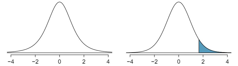
For the \(t\)-distribution with 3 degrees of freedom, as shown in the left panel of Figure 7.1.11, what should the value of \(t^{\star}\) be so that 95% of the area of the curve falls between -\(t^{\star}\) and +\(t^{\star}\text{?}\)
We can look at the column in the \(t\)-table that says 95% at the bottom row for the confidence level and trace it up to row \(df = 3\) to find that \(t^{\star} = 3.182\text{.}\)
A \(t\)-distribution with 20 degrees of freedom is shown in the right panel of Figure 7.1.11. Estimate the proportion of the distribution falling above 1.65.
We identify the row in the \(t\)-table using the degrees of freedom: \(df=20\text{.}\) Then we look for 1.65; it is not listed. It falls between the first and second columns. Since these values bound 1.65, their tail areas will bound the tail area corresponding to 1.65. We identify the one tail area of the first and second columns, 0.050 and 0.10, and we conclude that between 5% and 10% of the distribution is more than 1.65 standard deviations above the mean. If we like, we can identify the precise area using statistical software: 0.0573.
When the desired degrees of freedom is not listed on the table, choose a conservative value: round the degrees of freedom down, i.e. move up to the previous row listed. Another options is to use a calculator or statistical software to get a precise value.
When estimating the mean and standard deviation from a small sample, the \(t\)-distribution is a more accurate tool than the normal model. This is true for both small and large samples.
Use the \(t\)-distribution for inference of the sample mean when observations are independent and nearly normal. You may relax the nearly normal condition as the sample size increases. For example, the data distribution may be moderately skewed when the sample size is at least 30.
To proceed with the \(t\)-distribution for inference about a single mean, we must check two conditions.
Independence of observations. We verify this condition just as we did before. We collect a simple random sample from less than 10% of the population, or if it was an experiment or random process, we carefully check to the best of our abilities that the observations were independent.
\(n \gt 30\) or observations come from a nearly normal distribution. We can easily check if the sample size is at least 30. If it is not, then this second condition requires more care. We often (i) take a look at a graph of the data, such as a dot plot or box plot, for obvious departures from the normal model, and (ii) consider whether any previous experiences alert us that the data may not be nearly normal.
When examining a sample mean and estimated standard deviation from a sample of \(n\) independent and nearly normal observations, we use a \(t\)-distribution with \(n-1\) degrees of freedom (\(df\)). For example, if the sample size was 19, then we would use the \(t\)-distribution with \(df=19-1=18\) degrees of freedom and proceed exactly as we did in Chapter 5, except that now we use the \(t\)-table.
In general, when the population mean is uknown, the population standard deviation will also be unknown. When this is the case, we estimate the population standard deviation with the sample standard deviation and we use SE instead of SD.
When we use the sample standard deviation, we use the \(t\)-distribution with \(df=n-1\) degrees of freedom instead of the normal distribution.
When the sample size \(n\) is at least 30, the Central Limit Theorem tells us that we do not have to worry too much about skew in the data. When this is not true, we need verify that the observations come from a nearly normal distribution. In some cases, this may be known, such as if the population is the heights of adults.
What do we do, though, if the population is not known to be approximately normal AND the sample size is small? We must look at the distribution of the data and check for excessive skew.
We should exercise caution when verifying the normality condition for small samples. It is important to not only examine the data but also think about where the data come from. For example, ask: would I expect this distribution to be symmetric, and am I confident that outliers are rare?
You may relax the normality condition as the sample size goes up. If the sample size is 10 or more, slight skew is not problematic. Once the sample size hits about 30, then moderate skew is reasonable. Data with strong skew or outliers require a more cautious analysis.
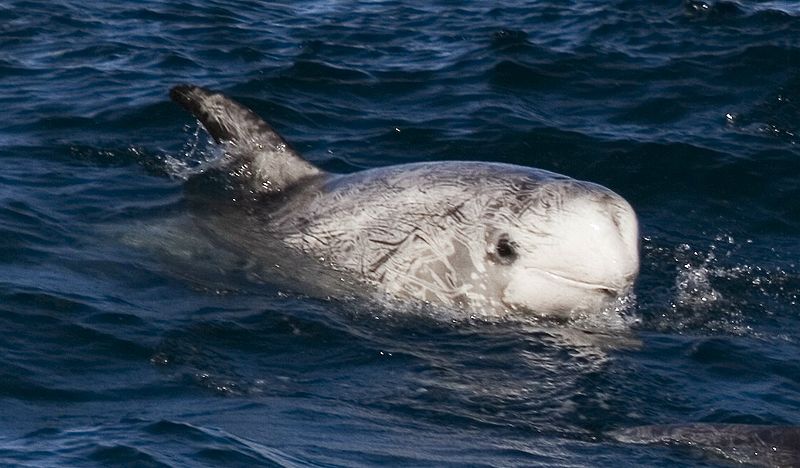
Dolphins are at the top of the oceanic food chain, which causes dangerous substances such as mercury to concentrate in their organs and muscles. This is an important problem for both dolphins and other animals, like humans, who occasionally eat them.
Here we identify a confidence interval for the average mercury content in dolphin muscle using a sample of 19 Risso's dolphins from the Taiji area in Japan. 2 Taiji was featured in the movie The Cove, and it is a significant source of dolphin and whale meat in Japan. Thousands of dolphins pass through the Taiji area annually, and we will assume these 19 dolphins represent a simple random sample from those dolphins. Data reference: Endo T and Haraguchi K. 2009. High mercury levels in hair samples from residents of Taiji, a Japanese whaling town. Marine Pollution Bulletin 60(5):743-747. The data are summarized in Table 7.1.13. The minimum and maximum observed values can be used to evaluate whether or not there are obvious outliers or skew.
| \(n\) | \(\bar{x}\) | \(s\) | minimum | maximum |
| 19 | 4.4 | 2.3 | 1.7 | 9.2 |
Are the independence and normality conditions satisfied for this data set?
The observations are a simple random sample and consist of less than 10% of the population, therefore independence is reasonable. To check the normality condition of the population, we would like to graph the data from the sample. However, we do not have all of the data. Instead, we will have to look at the summary statistics provided in Table 7.1.13. These summary statistics do not suggest any skew or outliers; all observations are within 2.5 standard deviations of the mean. Based on this evidence, the normality assumption seems reasonable.
In the normal model, we used \(z^{\star}\) and the standard deviation to determine the width of a confidence interval. We revise the confidence interval formula slightly when using the \(t\)-distribution:
3 \(t^{\star}_{df}\) Multiplication factor for \(t\)-intervalThe sample mean is computed just as before: \(\bar{x} = 4.4\text{.}\) In place of the standard deviation of \(\bar{x}\text{,}\) we use the standard error of \(\bar{x}\text{:}\) \(SE_{\bar{x}} = s/\sqrt{n} = 0.528\text{.}\)
The value \(t^{\star}_{df}\) is a cutoff we obtain based on the confidence level and the \(t\)-distribution with \(df\) degrees of freedom. Before determining this cutoff, we will first need the degrees of freedom.
If the sample has \(n\) observations and we are examining a single mean, then we use the \(t\)-distribution with \(df=n-1\) degrees of freedom.
In our current example, we should use the \(t\)-distribution with \(df=19-1=18\) degrees of freedom. Then identifying \(t_{18}^{\star}\) is similar to how we found \(z^{\star}\text{.}\)
For a 95% confidence interval, we want to find the cutoff \(t^{\star}_{18}\) such that 95% of the \(t\)-distribution is between -\(t^{\star}_{18}\) and \(t^{\star}_{18}\text{.}\)
We look in the \(t\)-table in Table 7.1.5, find the column with 95% along the bottom row and then the row with 18 degrees of freedom: \(t^{\star}_{18} = 2.10\text{.}\)
Generally the value of \(t^{\star}_{df}\) is slightly larger than what we would get under the normal model with \(z^{\star}\text{.}\)
Finally, we can substitute all our values into the confidence interval equation to create the 95% confidence interval for the average mercury content in muscles from Risso's dolphins that pass through the Taiji area:
We are 95% confident the true average mercury content of muscles in Risso's dolphins is between 3.29 and 5.51 \(\mu\)g/wet gram. This is above the Japanese regulation level of 0.4 \(\mu\)g/wet gram.
Based on a sample of \(n\) independent and nearly normal observations, a confidence interval for the population mean is
where \(\bar{x}\) is the sample mean, \(t^{\star}_{df}\) corresponds to the confidence level and degrees of freedom, and \(SE\) is the standard error given by \(\frac{s}{\sqrt{n}}\text{.}\)
State the name of the CI being used.
1-sample \(t\)-interval.
Verify conditions.
A simple random sample.
Population is known to be normal OR \(n\ge 30\) OR graph of sample is approximately symmetric with no outliers, making the assumption that the population is normal a reasonable one.
Plug in the numbers and write the interval in the form
The point estimate is \(\bar{x}\)
\(df = n-1\)
Plug in a critical value \(t^\star\) using the \(t\)-table at row\(=n-1\)
Use \(SE = \frac{s}{\sqrt{n}}\)
Evaluate the CI and write in the form ( \(\_\) , \(\_\) )
Interpret the interval: ``We are [XX]% confident that the true average of [...] is between [...] and [...]."
State the conclusion to the original question.
The FDA's webpage provides some data on mercury content of fish. 4 https://www.fda.gov/food/foodborneillnesscontaminants/metals/ucm115644.htm Based on a sample of 15 croaker white fish (Pacific), a sample mean and standard deviation were computed as 0.287 and 0.069 ppm (parts per million), respectively. The 15 observations ranged from 0.18 to 0.41 ppm. We will assume these observations are independent. Construct an appropriate 95% confidence interval for the true average mercury content of croaker white fish (Pacific). Is there evidence that the average mercury content is greater than 0.275 ppm? 5 The interval called for in this problem is a 1-sample \(t\)-interval. We will assume that the sample was random. \(n\) is small, but there are no obvious outliers; all observations are within 2 standard deviations of the mean. If there is skew, it is not evident. Therefore we do not have reason to believe the mercury content in the population is not nearly normal in this type of fish. We can now identify and calculate the necessary quantities. The point estimate is the sample average, which is 0.287. The standard error: \(SE = \frac{0.069}{\sqrt{15}} = 0.0178\text{.}\) Degrees of freedom: \(df = n - 1 = 14\text{.}\) Using the \(t\)-table, we identify \(t^{\star}_{14} = 2.145\text{.}\) The confidence interval is given by: \(0.287 \ \pm\ 2.145\times 0.0178\ \to\ (0.249, 0.325)\text{.}\) We are 95% confident that the true average mercury content of croaker white fish (Pacific) is between 0.249 and 0.325 ppm. Because the interval contains 0.275 as well as value less than 0.275, we do not have evidence that the true average mercury content is greater than 0.275, even though our sample average was 0.287.
Many companies are concerned about rising healthcare costs. A company may estimate certain health characteristics of its employees, such as blood pressure, to project its future cost obligations. However, it might be too expensive to measure the blood pressure of every employee at a large company, and the company may choose to take a sample instead.
Blood pressure oscillates with the beating of the heart, and the systolic pressure is defined as the peak pressure when a person is at rest. The average systolic blood pressure for people in the U.S. is about 130 mmHg with a standard deviation of about 25 mmHg. How large of a sample is necessary to estimate the average systolic blood pressure with a margin of error of 4 mmHg using a 95% confidence level?
The challenge in this case is to find the sample size \(n\) so that this margin of error is less than or equal to \(m = 4\text{,}\) which we write as an inequality:-1mm
To proceed and solve for \(n\text{,}\) we substitute the best estimate we have for \(\sigma_{employee}\text{:}\) 25.
The minimum sample size that meets the condition is 151. We round up because the sample size must be an integer and it must be greater than or equal to 150.06.
A potentially controversial part of Example 7.1.16 is the use of the U.S. standard deviation for the employee standard deviation. Usually the standard deviation is not known. In such cases, it is reasonable to review scientific literature or market research to make an educated guess about the standard deviation.
The margin of error for a sample mean is similar to the formula we add and subtract in a confidence interval:
The value \(z^{\star}\) is chosen to correspond to the desired confidence level, and \(\sigma\) is the standard deviation associated with the population.
To estimate the necessary sample size to achieve a margin of error of \(m\text{,}\) we require the margin of error \(ME\) to be less than or equal to \(m\text{:}\)
We solve for the sample size, \(n\text{.}\)
Sample size computations are helpful in planning data collection, and they require careful forethought.
Is the typical US runner getting faster or slower over time? We consider this question in the context of the Cherry Blossom Run, comparing runners in 2006 and 2012. Technological advances in shoes, training, and diet might suggest runners would be faster in 2012. An opposing viewpoint might say that with the average body mass idx on the rise, people tend to run slower. In fact, all of these components might be influencing run time.
The average time for all runners who finished the Cherry Blossom Run in 2006 was 93.29 minutes (93 minutes and about 17 seconds). We want to determine using data from 100 participants in the 2012 Cherry Blossom Run whether runners in this race are getting faster or slower, versus the other possibility that there has been no change.
What are appropriate hypotheses for this context? 6 \(H_0\text{:}\) The average 10 mile run time in 2012 was the same as in 2006 (93.29 minutes). \(\mu = 93.29\text{.}\) \(H_A\text{:}\) The average 10 mile run time for 2012 was different than 93.29 minutes. \(\mu \neq 93.29\text{.}\)
The data come from a simple random sample from less than 10% of all participants, so the observations are independent. However, should we be worried about skew in the data? A histogram of the times is shown in Figure 7.1.19. 7 Since the sample size 100 is greater than 30, we do not need to worry about slight skew in the data.
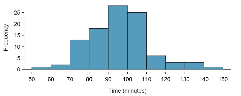
time for a single sample of size 100.With independence satisfied and skew not a concern, we can proceed with performing a hypothesis test using the \(t\)-distribution.
The sample mean and sample standard deviation are 95.61 and 15.78 minutes, respectively. Recall that the sample size is 100. What is the p-value for the test, and what is your conclusion? 8 With the conditions satisfied for the \(t\)-distribution, we can compute the standard error (\(SE = 15.78 / \sqrt{100} = 1.58\) and the T score: \(T = \frac{95.61 - 93.29}{1.58} = 1.47\text{.}\) For \(df = 100 - 1 = 99\text{,}\) we would find a p-value between 0.10 and 0.20 (two-sided!). Because the p-value is greater than 0.05, we do not reject the null hypothesis. That is, the data do not provide strong evidence that the average run time for the Cherry Blossom Run in 2012 is any different than the 2006 average.
State the name of the test being used.
1-sample \(t\)-test.
Verify conditions.
Data come from a simple random sample.
Population is known to be normal OR \(n\ge 30\) OR graph of data is approximately symmetric with no outliers, making the assumption that population is normal a reasonable one.
Write the hypotheses in plain language, then set them up in mathematical notation.
H\(_0: \mu = \mu_0\)
H\(_0: \mu \ne \text{ or } \lt \text{ or } > \mu_0\)
Identify the significance level \(\alpha\text{.}\)
Calculate the test statistic and \(df\text{:}\) \(T = \frac{\text{ point estimate } - \text{ null value } }{\text{ SE of estimate } }\)
The point estimate is \(\bar{x}\)
\(SE = \frac{s}{\sqrt{n}}\)
\(df=n-1\)
Find the p-value, compare it to \(\alpha\text{,}\) and state whether to reject or not reject the null hypothesis.
Write the conclusion in the context of the question.
Recall the example about the mercury content in croaker white fish (Pacific). Based on a sample of 15, a sample mean and standard deviation were computed as 0.287 and 0.069 ppm (parts per million), respectively. Carry out an appropriate test to determine if 0.25 is a reasonable value for the average mercury content. 9 We should carry out a 1-sample \(t\)-test. The conditions have already been checked. \(H_0: \mu=0.25\text{;}\) The true average mercury content is 0.25 ppm. \(H_A: \mu \ne 0.25\text{;}\) The true average mercury content is not equal to 0.25 ppm. Let \(\alpha=0.05\text{.}\) \(SE = \frac{0.069}{\sqrt{15}} = 0.0178\text{.}\) \(T=\frac{0.287-0.25}{0.0178}=2.07\) \(df=15-1=14\text{.}\) p-value\(=0.057>0.05\text{,}\) so we do not reject the null hypothesis. We do not have sufficient evidence that the average mercury content in croaker white fish is not 0.25.
Recall that the 95% confidence interval for the average mercuy content in croaker white fish was (0.249, 0.325). Discuss whether the conclusion of the test of hypothesis is consistent or inconsistent with the conclusion of the hypothesis test.
It is consistent because 0.25 is located (just barely) inside the confidence interval, so it is a reasonable value. Our hypothesis test did not reject the hypothesis that \(\mu=0.25\text{,}\) implying that it is a plausible value. Note, though, that the hypothesis test did not prove that \(\mu=.25\text{.}\) A hypothesis cannot prove that the mean is a specific value. It can only find evidence that it is not a specific value. Note also that the p-value was close to the cutoff of 0.05. This is because the value 0.25 was close to edge of the confidence interval.
MISSINGVIDEOLINK Use STAT, TESTS, T-Test.
Choose STAT.
Right arrow to TESTS.
Down arrow and choose 2:T-Test.
Choose Data if you have all the data or Stats if you have the mean and standard deviation.
Let \(\mu_0\) be the null or hypothesized value of \(\mu\text{.}\)
If you choose Data, let List be L1 or the list in which you entered your data (don't forget to enter the data!) and let Freq be 1.
If you choose Stats, enter the mean, SD, and sample size.
Choose \(\ne\text{,}\) \(\lt\text{,}\) or \(\gt\) to correspond to H\(_A\text{.}\)
Choose Calculate and hit ENTER, which returns:
t |
t statistic | Sx |
the sample standard deviation | |
p |
p-value | n |
the sample size | |
| \(\bar{x}\) | the sample mean |
MISSINGVIDEOLINK
Navigate to STAT (MENU button, then hit the 2 button or select STAT).
If necessary, enter the data into a list.
Choose the TEST option (F3 button).
Choose the t option (F2 button).
Choose the 1-S option (F1 button).
Choose either the Var option (F2) or enter the data in using the List option.
Specify the test details:
Specify the sidedness of the test using the F1, F2, and F3 keys.
Enter the null value, \(\mu\)0.
If using the Var option, enter the summary statistics. If using List, specify the list and leave Freq values at 1.
Hit the EXE button, which returns
| alternative hypothesis | \(\bar{x}\) | sample mean | ||
t |
T statistic | sx |
sample standard deviation | |
p |
p-value | n |
sample size |
MISSINGVIDEOLINK Use STAT, TESTS, TInterval.
Choose STAT.
Right arrow to TESTS.
Down arrow and choose 8:TInterval.
Choose Data if you have all the data or Stats if you have the mean and standard deviation.
If you choose Data, let List be L1 or the list in which you entered your data (don't forget to enter the data!) and let Freq be 1.
If you choose Stats, enter the mean, SD, and sample size.
Let C-Level be the desired confidence level.
Choose Calculate and hit ENTER, which returns:
(,) |
the confidence interval |
| \(\bar{x}\) | the sample mean |
Sx |
the sample SD |
n |
the sample size |
MISSINGVIDEOLINK
Navigate to STAT (MENU button, then hit the 2 button or select STAT).
If necessary, enter the data into a list.
Choose the INTR option (F3 button), t (F2 button), and 1-S (F1 button).
Choose either the Var option (F2) or enter the data in using the List option.
Specify the interval details:
Confidence level of interest for C-Level.
If using the Var option, enter the summary statistics. If using List, specify the list and leave Freq value at 1.
Hit the EXE button, which returns
Left, Right
|
ends of the confidence interval |
| \(\bar{x}\) | sample mean |
sx |
sample standard deviation |
n |
sample size |
The average time for all runners who finished the Cherry Blossom Run in 2006 was 93.29 minutes. In 2012, the average time for 100 randomly selected participants was 95.61, with a standard deviation of 15.78 minutes. Use a calculator to find the \(T\) statistic and p-value for the appropriate test to see if the average time for the participants in 2012 is different than it was in 2006. 10 Let \(\mu_0\) be 93.29. Choose \(\neq\) to correspond to \(H_A\text{.}\) \(T=1.47\text{,}\) \(df = 99\text{,}\) and p-value\(=0.14\text{.}\)
Use a calculator to find a 95% confidence interval for the average run time for participants in the 2012 Cherry Blossum Run using the sample data: \(\bar{x} = 95.61\) minutes, \(s = 15.78\) minutes, and the sample size was 100. 11 The interval is \((92.52, 98.70)\text{.}\)