
Section 8.4 Inference for the slope of a regression line
¶Open Intro: Inference for Linear Regression
In this section we discuss uncertainty in the estimates of the slope and y-intercept for a regression line. Just as we identified standard errors for point estimates in previous chapters, we first discuss standard errors for these new estimates. However, in the case of regression, we will identify standard errors using statistical software.
Subsection 8.4.1 Midterm elections and unemployment
Elections for members of the United States House of Representatives occur every two years, coinciding every four years with the U.S. Presidential election. The set of House elections occurring during the middle of a Presidential term are called midterm elections. In America's two-party system, one political theory suggests the higher the unemployment rate, the worse the President's party will do in the midterm elections.
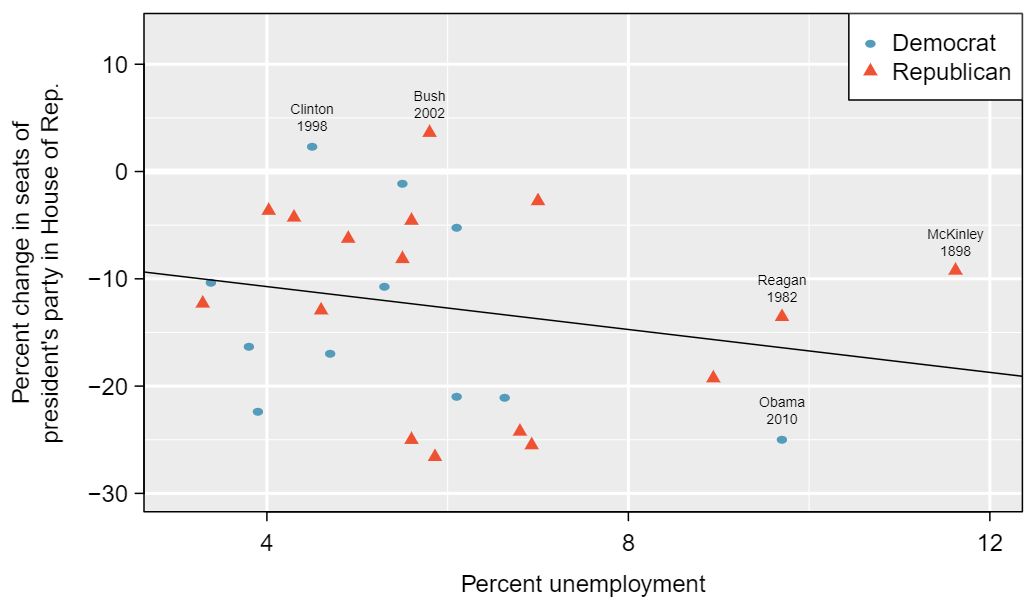
To assess the validity of this claim, we can compile historical data and look for a connection. We consider every midterm election from 1898 to 2010, with the exception of those elections during the Great Depression. Figure 8.4.2 shows these data and the least-squares regression line:
\begin{gather*}
\text{ % change in House seats for President's party }\\
= -6.71 - 1.00\times \text{ (unemployment rate) }
\end{gather*}
We consider the percent change in the number of seats of the President's party (e.g. percent change in the number of seats for Democrats in 2010) against the unemployment rate.
Examining the data, there are no clear deviations from linearity, the constant variance condition, or in the normality of residuals (though we don't examine a normal probability plot here). While the data are collected sequentially, a separate analysis was used to check for any apparent correlation between successive observations; no such correlation was found.
The data for the Great Depression (1934 and 1938) were removed because the unemployment rate was 21% and 18%, respectively. Do you agree that they should be removed for this investigation? Why or why not? 1 We will provide two considerations. Each of these points would have very high leverage on any least-squares regression line, and years with such high unemployment may not help us understand what would happen in other years where the unemployment is only modestly high. On the other hand, these are exceptional cases, and we would be discarding important information if we exclude them from a final analysis.
There is a negative slope in the line shown in Figure 8.4.2. However, this slope (and the y-intercept) are only estimates of the parameter values. We might wonder, is this convincing evidence that the “true” linear model has a negative slope? That is, do the data provide strong evidence that the political theory is accurate? We can frame this investigation into a one-sided statistical hypothesis test:
\(H_0: \beta_1 = 0\text{.}\) The true linear model has slope zero.
\(H_A: \beta_1 \lt 0\text{.}\) The true linear model has a slope less than zero. The higher the unemployment, the greater the loss for the President's party in the House of Representatives.
We would reject \(H_0\) in favor of \(H_A\) if the data provide strong evidence that the true slope parameter is less than zero. To assess the hypotheses, we identify a standard error for the estimate, compute an appropriate test statistic, and identify the p-value.
Subsection 8.4.2 Understanding regression output from software
¶Just like other point estimates we have seen before, we can compute a standard error and test statistic for \(b_1\text{.}\) We will generally label the test statistic using a \(T\text{,}\) since it follows the \(t\)-distribution.
TIP: Hypothesis tests on the slope of the regression line
Use a \(t\)-test with \(n - 2\) degrees of freedom when performing a hypothesis test on the slope of a regression line.
We will rely on statistical software to compute the standard error and leave the explanation of how this standard error is determined to a second or third statistics course. The table below shows software output for the least squares regression line in Figure 8.4.2. The row labeled unemp represents the information for the slope, which is the coefficient of the unemployment variable.
The regression equation is:

Change = -6.7142 - 1.0010 unemp

Predictor      Coef   SE Coef       T        P

Constant    -6.7142    5.4567   -1.23   0.2300

unemp       -1.0010    0.8717   -1.15   0.2617

S = 9.624   R-Sq = 0.03%    R-Sq(adj) = -3.7%
Example 8.4.4
What do the first and second columns of numbers in the regression summary represent?
Solution
The entries in the first column represent the least squares estimates, \(b_0\) and \(b_1\text{,}\) and the values in the second column correspond to the standard errors of each estimate.
We previously used a \(T\) test statistic for hypothesis testing in the context of numerical data. Regression is very similar. In the hypotheses we consider, the null value for the slope is 0, so we can compute the test statistic using the \(T\) score formula:
\begin{gather*}
T = \frac{\text{ estimate } - \text{ null value } }{\text{ SE } } = \frac{-1.0010 - 0}{0.8717} = -1.15
\end{gather*}
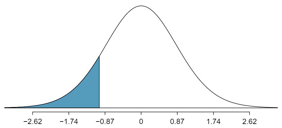
We can look for the one-sided p-value — shown in Figure 8.4.5 — using the probability table for the \(t\)-distribution in Appendix C.
Example 8.4.6
In this example, the sample size \(n=27\text{.}\) Identify the degrees of freedom and p-value for the hypothesis test.
Solution
The degrees of freedom for this test is \(n-2\text{,}\) or \(df = 27-2 = 25\text{.}\) Looking in the 25 degrees of freedom row in Appendix C, we see that the absolute value of the test statistic is smaller than any value listed, which means the tail area and therefore also the p-value is larger than 0.100 (one tail!). Because the p-value is so large, we fail to reject the null hypothesis. That is, the data do not provide convincing evidence that a higher unemployment rate has any correspondence with smaller or larger losses for the President's party in the House of Representatives in midterm elections.
We could have identified the \(T\) test statistic from the software output of the regression model, shown in the unemp row and third column (t value). The entry in the unemp row and last column represents the p-value for the two-sided hypothesis test where the null value is zero. The corresponding one-sided test would have a p-value half of the listed value.
Inference for regression
We usually rely on statistical software to identify point estimates and standard errors for parameters of a regression line. After verifying conditions hold for fitting a line, we can use the methods learned in Section 7.1 for the \(t\)-distribution to create confidence intervals for regression parameters or to evaluate hypothesis tests.
Caution: Don't carelessly use the p-value from regression output
The last column in regression output often lists p-values for one particular hypothesis: a two-sided test where the null value is zero. If your test is one-sided and the point estimate is in the direction of \(H_A\text{,}\) then you can halve the software's p-value to get the one-tail area. If neither of these scenarios match your hypothesis test, be cautious about using the software output to obtain the p-value.
Example 8.4.7
Examine Figure 8.2.14, which relates the Elmhurst College aid and student family income. How sure are you that the slope is statistically significantly different from zero? That is, do you think a formal hypothesis test would reject the claim that the true slope of the line should be zero?
Solution
While the relationship between the variables is not perfect, there is an evident decreasing trend in the data. This suggests the hypothesis test will reject the null claim that the slope is zero.
Recall that \(b_1=r\frac{s_y}{s_x}\text{.}\) If the slope of the true regression line is zero, the population correlation coefficient must also be zero. The linear regression test for \(\beta_1=0\) is equivalent, then, to a test for the population correlation coefficient \(\rho=0\text{.}\)
Guided Practice 8.4.8
The regression summary below shows statistical software output from fitting the least squares regression line shown in Figure 8.2.14. Use this output to formally evaluate the following hypotheses. \(H_0\text{:}\) The true slope of the regression line is zero. \(H_A\text{:}\) The true slope of the regression line is not zero. 2 We look in the second row corresponding to the family income variable. We see the point estimate of the slope of the line is -0.0431, the standard error of this estimate is 0.0108, and the \(T\) test statistic is -3.98. The p-value corresponds exactly to the two-sided test we are interested in: 0.0002. The p-value is so small that we reject the null hypothesis and conclude that family income and financial aid at Elmhurst College for freshman entering in the year 2011 are negatively correlated and the true slope parameter is indeed less than 0, just as we believed in Example 8.4.7.
       The regression equation is:

       aid = 24.31933 - 0.04307 family_income

       Predictor        Coef        SE Coef   T        P

       Constant         24.31933    1.29145   18.831   < 2e-16

       family_income   -0.04307    0.01081   -3.985   0.000229

       S = 4.783   R-Sq = 24.86%    R-Sq(adj) = 23.29%
Always check assumptions
If conditions for fitting the regression line do not hold, then the methods presented here should not be applied. The standard error or distribution assumption of the point estimate — assumed to be normal when applying the \(T\) test statistic — may not be valid.
Subsection 8.4.3 Summarizing inference procedures for linear regression
Hypothesis test for the slope of regression line
-
State the name of the test being used.
Linear regression \(t\)-test
-
Verify conditions.
The residual plot has no pattern.
-
Write the hypotheses in plain language. No mathematical notation is needed for this test.
H\(_0\text{:}\) \(\beta_1=0\text{,}\) There is no significant linear relationship between [x] and [y].
H\(_A\text{:}\) \(\beta_1 \ne,\text{ or } \lt , \text{ or } >0\text{,}\) There is a significant or significant negative or significant positive linear relationship between [x] and [y].
Identify the significance level \(\alpha\text{.}\)
-
Calculate the test statistic and \(df\text{:}\) \(T = \frac{\text{ point estimate } - \text{ null value } }{\text{ SE of estimate } }\)
The point estimate is \(b_1\)
\(SE\) can be located on regression summary table next to value of \(b_1\)
\(df = n-2\)
Find the p-value, compare it to \(\alpha\text{,}\) and state whether to reject or not reject the null hypothesis.
Write the conclusion in the context of the question.
Constructing a confidence interval for the slope of regression line
-
State the name of the CI being used.
\(t\)-interval for slope of regression line
-
Verify conditions.
The residual plot has no pattern.
-
Plug in the numbers and write the interval in the form
\begin{equation*} \text{ point estimate } \pm t^\star \times \text{ SE of estimate } \end{equation*}The point estimate is \(b_1\text{.}\)
\(df = n-2\)
The critical value \(t^*\) can be found on the \(t\)-table at row \(df = n-2\)
\(SE\) can be located on regression summary table next to value of \(b_1\)
Evaluate the CI and write in the form ( \(\_\) , \(\_\) ).
Interpret the interval: “We are [XX]% confident that this interval contains the true average increase in [y] for each additional [unit] of [x].”
State the conclusion to the original question.
Subsection 8.4.4 Calculator: the linear regression \(t\)-test and \(t\)-interval
When doing this type of inference, we generally make use of computer output that provides us with the necessary quantities: \(b\) and \(s_b\text{.}\) The calculator functions below require knowing all of the data and are, therefore, rarely used. We describe them here for the sake of completion.
TI-83/84: Linear regression \(t\)-test on \(\beta_1\)
MISSINGVIDEOLINK Use STAT, TESTS, LinRegTTest.
Choose
STAT.Right arrow to
TESTS.Down arrow and choose
F:LinRegTest. (On TI-83 it isE:LinRegTTest).Let
XlistbeL1andYlistbeL2. (Don't forget to enter the \(x\) and \(y\) values inL1andL2before doing this test.)Let
Freqbe1.Choose \(\ne\text{,}\) \(\lt\text{,}\) or \(\gt\) to correspond to H\(_A\text{.}\)
Leave
RegEQblank.Choose
Calculateand hitENTER, which returns:tt statistic b\(b_1\text{,}\) slope of the line pp-value sst. dev. of the residuals dfdegrees of freedom for the test \(r^2\) \(R^2\text{,}\) explained variance a\(b_0\text{,}\) y-intercept of the line r\(r\text{,}\) correlation coefficient
Casio fx-9750GII: Linear regression \(t\)-test on \(\beta_1\)
MISSINGVIDEOLINK
Navigate to
STAT(MENUbutton, then hit the2button or selectSTAT).Enter your data into 2 lists.
Select
TEST(F3),t(F2), andREG(F3).If needed, update the sidedness of the test and the
XListandYListlists. TheFreqshould be set to1.Hit
EXE, which returns:tt statistic b\(b_1\text{,}\) slope of the line pp-value sst. dev. of the residuals dfdegrees of freedom for the test r\(r\text{,}\) correlation coefficient a\(b_0\text{,}\) y-intercept of the line \(r^2\) \(R^2\text{,}\) explained variance
TI-84: \(t\)-interval for \(\beta_1\)
MISSINGVIDEOLINK Use STAT, TESTS, LinRegTInt.
Choose
STAT.Right arrow to
TESTS.-
Down arrow and choose
G:LinRegTest.This test is not built into the TI-83.
Let
XlistbeL1andYlistbeL2. (Don't forget to enter the \(x\) and \(y\) values inL1andL2before doing this interval.)Let
Freqbe1.Enter the desired confidence level.
Leave
RegEQblank.Choose
Calculateand hitENTER, which returns:(,)the confidence interval b\(b_1\text{,}\) the slope of best fit line of the sample data dfdegrees of freedom associated with this confidence interval sstandard deviation of the residuals a\(b_0\text{,}\) the y-intercept of the best fit line of the sample data \(r^2\) \(R^2\text{,}\) the explained variance r\(r\text{,}\) the correlation coefficient