Advanced High School Statistics: First Edition

1 Identify the critical \(t\)

An independent random sample is selected from an approximately normal population with unknown standard deviation. Find the degrees of freedom and the critical \(t\)-value (t\(^\star\)) for the given sample size and confidence level.

1. \(n = 6\text{,}\) CL = 90 Answer

   \(df=6-1=5\text{,}\) \(t_{5}^{\star} = 2.02\) (column with two tails of 0.10, row with \(df=5\)).

2. \(n = 21\text{,}\) CL = 98 Answer

   \(df=21-1=20\text{,}\) \(t_{20}^{\star} = 2.53\) (column with two tails of 0.02, row with \(df=20\)).

3. \(n = 29\text{,}\) CL = 95 Answer

   \(df=28\text{,}\) \(t_{28}^{\star} = 2.05\text{.}\)

4. \(n = 12\text{,}\) CL = 99 Answer

   \(df=11\text{,}\) \(t_{11}^{\star} = 3.11\text{.}\)

2 \(t\)-distribution

The figure below shows three unimodal and symmetric curves: the standard normal (z) distribution, the \(t\)-distribution with 5 degrees of freedom, and the \(t\)-distribution with 1 degree of freedom. Determine which is which, and explain your reasoning.

3 Find the p-value, Part I

An independent random sample is selected from an approximately normal population with an unknown standard deviation. Find the p-value for the given set of hypotheses and \(T\) test statistic. Also determine if the null hypothesis would be rejected at \(\alpha = 0.05\text{.}\)

1. \(H_A: \mu \gt \mu_0\text{,}\) \(n = 11\text{,}\) \(T = 1.91\) Answer

   between 0.025 and 0.05

2. \(H_A: \mu \lt \mu_0\text{,}\) \(n = 17\text{,}\) \(T = -3.45\) Answer

   less than 0.005

3. \(H_A: \mu \ne \mu_0\text{,}\) \(n = 7\text{,}\) \(T = 0.83\) Answer

   greater than 0.2

4. \(H_A: \mu \gt \mu_0\text{,}\) \(n = 28\text{,}\) \(T = 2.13\) Answer

   between 0.01 and 0.025

4 Find the p-value, Part II

An independent random sample is selected from an approximately normal population with an unknown standard deviation. Find the p-value for the given set of hypotheses and \(T\) test statistic. Also determine if the null hypothesis would be rejected at \(\alpha = 0.01\text{.}\)

1. \(H_A: \mu \gt 0.5\text{,}\) \(n = 26\text{,}\) \(T = 2.485\)

2. \(H_A: \mu \lt 3\text{,}\) \(n = 18\text{,}\) \(T = 0.5\)

5 Working backwards, Part I

A 95% confidence interval for a population mean, \(\mu\text{,}\) is given as (18.985, 21.015). This confidence interval is based on a simple random sample of 36 observations. Calculate the sample mean and standard deviation. Assume that all conditions necessary for inference are satisfied. Use the \(t\)-distribution in any calculations.

6 Working backwards, Part II

A 90% confidence interval for a population mean is (65, 77). The population distribution is approximately normal and the population standard deviation is unknown. This confidence interval is based on a simple random sample of 25 observations. Calculate the sample mean, the margin of error, and the sample standard deviation.

7 Sleep habits of New Yorkers

New York is known as “the city that never sleeps”. A random sample of 25 New Yorkers were asked how much sleep they get per night. Statistical summaries of these data are shown below. Do these data provide strong evidence that New Yorkers sleep less than 8 hours a night on average?

1. Write the hypotheses in symbols and in words. Answer

   \(H_0\text{:}\) \(\mu = 8\) (New Yorkers sleep 8 hrs per night on average.) \(H_A\text{:}\) \(\mu \lt 8\) (New Yorkers sleep less than 8 hrs per night on average.)

2. Check conditions, then calculate the test statistic, \(T\text{,}\) and the associated degrees of freedom. Answer

   Independence: The sample is random and from less than 10% of New Yorkers. The sample is small, so we will use a \(t\) distribution. For this size sample, slight skew is acceptable, and the min/max suggest there is not much skew in the data. \(T = -1.75\text{.}\) \(df=25-1=24\text{.}\)

3. Find and interpret the p-value in this context. Drawing a picture may be helpful. Answer

   \(0.025 \lt\) p-value \(\lt0.05\text{.}\) If in fact the true population mean of the amount New Yorkers sleep per night was 8 hours, the probability of getting a random sample of 25 New Yorkers where the average amount of sleep is 7.73 hrs per night or less is between 0.025 and 0.05.

4. What is the conclusion of the hypothesis test? Answer

   Since p-value \(\gt\) 0.05, reject \(H_0\text{.}\) The data provide strong evidence that New Yorkers sleep less than 8 hours per night on average.

5. If you were to construct a 90% confidence interval that corresponded to this hypothesis test, would you expect 8 hours to be in the interval? Answer

   No, as we rejected \(H_0\text{.}\)

8 Fuel efficiency of Prius

Fueleconomy.gov, the official US government source for fuel economy information, allows users to share gas mileage information on their vehicles. The histogram below shows the distribution of gas mileage in miles per gallon (MPG) from 14 users who drive a 2012 Toyota Prius. The sample mean is 53.3 MPG and the standard deviation is 5.2 MPG. Note that these data are user estimates and since the source data cannot be verified, the accuracy of these estimates are not guaranteed.¹\footfullcite LINK IF NEEDED{data:prius}

1. We would like to use these data to evaluate the average gas mileage of all 2012 Prius drivers. Do you think this is reasonable? Why or why not?

2. The EPA claims that a 2012 Prius gets 50 MPG (city and highway mileage combined). Do these data provide strong evidence against this estimate for drivers who participate on fueleconomy.gov? Note any assumptions you must make as you proceed with the test.

3. Calculate a 95% confidence interval for the average gas mileage of a 2012 Prius by drivers who participate on fueleconomy.gov.

9 Find the mean

You are given the following hypotheses:

We know that the sample standard deviation is 8 and the sample size is 20. For what sample mean would the p-value be equal to 0.05? Assume that all conditions necessary for inference are satisfied.

10 \(t^{\star}\) vs.\(z^{\star}\)

For a given confidence level, \(t^{\star}_{df}\) is larger than \(z^{\star}\text{.}\) Explain how \(t^{*}_{df}\) being slightly larger than \(z^{*}\) affects the width of the confidence interval.

11 Play the piano

Georgianna claims that in a small city renowned for its music school, the average child takes at least 5 years of piano lessons. We have a random sample of 20 children from the city, with a mean of 4.6 years of piano lessons and a standard deviation of 2.2 years.

1. Evaluate Georgianna's claim using a hypothesis test. Answer

   We will conduct a 1-sample \(t\)-test. \(H_0\text{:}\) \(\mu = 5\text{.}\) \(H_A\text{:}\) \(\mu \lt 5\text{.}\) We'll use \(\alpha = 0.05\text{.}\) This is a random sample, so the observations are independent. To proceed, we assume the distribution of years of piano lessons is approximately normal. \(SE = 2.2 / \sqrt{20} = 0.4919\text{.}\) The test statistic is \(T = (4.6 - 5) / SE = -0.81\text{.}\) \(df = 20 - 1 = 19\text{.}\) The one-tail p-value is about 0.21, which is bigger than \(\alpha = 0.05\text{,}\) so we do not reject \(H_0\text{.}\) That is, we do not have sufficiently strong evidence to reject Georgianna's claim.

2. Construct a 95% confidence interval for the number of years students in this city take piano lessons, and interpret it in context of the data. Answer

   Using \(SE = 0.4919\) and \(t_{df = 19}^{\star} = 2.093\text{,}\) the confidence interval is (3.57, 5.63). We are 95% confident that the average number of years a child takes piano lessons in this city is 3.57 to 5.63 years.

3. Do your results from the hypothesis test and the confidence interval agree? Explain your reasoning. Answer

   They agree, since we did not reject the null hypothesis and the null value of 5 was in the \(t\)-interval.

12 Auto exhaust and lead exposure

Researchers interested in lead exposure due to car exhaust sampled the blood of 52 police officers subjected to constant inhalation of automobile exhaust fumes while working traffic enforcement in a primarily urban environment. The blood samples of these officers had an average lead concentration of 124.32 \(\mu\)g/l and a SD of 37.74 \(\mu\)g/l; a previous study of individuals from a nearby suburb, with no history of exposure, found an average blood level concentration of 35 \(\mu\)g/l.²WI Mortada et al. “Study of lead exposure from automobile exhaust as a risk for nephrotoxicity among traffic policemen.” In: merican journal of nephrology 21.4 (2000), pp. 274-279.

1. Write down the hypotheses that would be appropriate for testing if the police officers appear to have been exposed to a higher concentration of lead.

2. Explicitly state and check all conditions necessary for inference on these data.

3. Test the hypothesis that the downtown police officers have a higher lead exposure than the group in the previous study. Interpret your results in context.

4. Based on your preceding result, without performing a calculation, would a 99% confidence interval for the average blood concentration level of police officers contain 35 \(\mu\)g/l?

13 Car insurance savings

A market researcher wants to evaluate car insurance savings at a competing company. Based on past studies he is assuming that the standard deviation of savings is $100. He wants to collect data such that he can get a margin of error of no more than $10 at a 95% confidence level. How large of a sample should he collect?

14 SAT scores

SAT scores of students at an Ivy League college are distributed with a standard deviation of 250 points. Two statistics students, Raina and Luke, want to estimate the average SAT score of students at this college as part of a class project. They want their margin of error to be no more than 25 points.

1. Raina wants to use a 90% confidence interval. How large a sample should she collect?

2. Luke wants to use a 99% confidence interval. Without calculating the actual sample size, determine whether his sample should be larger or smaller than Raina's, and explain your reasoning.

3. Calculate the minimum required sample size for Luke.

15 Air quality

Air quality measurements were collected in a random sample of 25 country capitals in 2013, and then again in the same cities in 2014. We would like to use these data to compare average air quality between the two years.

1. Should we use a one-sided or a two-sided test? Explain your reasoning. Answer

   Two-sided, we are evaluating a difference, not in a particular direction.

2. Should we use a paired or non-paired test? Explain your reasoning. Answer

   Paired, data are recorded in the same cities at two different time points. The temperature in a city at one point is not independent of the temperature in the same city at another time point.

3. Should we use a \(t\)-test or a z-test? Explain your reasoning. Answer

   \(t\)-test, sample is small and population standard deviation is unknown.

16 True / False: paired

Determine if the following statements are true or false. If false, explain.

1. In a paired analysis we first take the difference of each pair of observation, and then we do inference on these differences.

2. Two data sets of different sizes cannot be analyzed as paired data.

3. Each observation in one data set has a natural correspondence with exactly one observation from the other data set.

4. Each observation in one data set is subtracted from the average of the other data set's observations.

17 Paired or not, Part I?

In each of the following scenarios, determine if the data are paired.

1. Compare pre- (beginning of semester) and post-test (end of semester) scores of students. Answer

   Since it's the same students at the beginning and the end of the semester, there is a pairing between the datasets, for a given student their beginning and end of semester grades are dependent.

2. Assess gender-related salary gap by comparing salaries of randomly sampled men and women. Answer

   Since the subjects were sampled randomly, each observation in the men's group does not have a special correspondence with exactly one observation in the other (women's) group.

3. Compare artery thicknesses at the beginning of a study and after 2 years of taking Vitamin E for the same group of patients. Answer

   Since it's the same subjects at the beginning and the end of the study, there is a pairing between the datasets, for a subject student their beginning and end of semester artery thickness are dependent.

4. Assess effectiveness of a diet regimen by comparing the before and after weights of subjects. Answer

   Since it's the same subjects at the beginning and the end of the study, there is a pairing between the datasets, for a subject student their beginning and end of semester weights are dependent.

18 Paired or not, Part II?

In each of the following scenarios, determine if the data are paired.

1. We would like to know if Intel's stock and Southwest Airlines' stock have similar rates of return. To find out, we take a random sample of 50 days, and record Intel's and Southwest's stock on those same days.

2. We randomly sample 50 items from Target stores and note the price for each. Then we visit Walmart and collect the price for each of those same 50 items.

3. A school board would like to determine whether there is a difference in average SAT scores for students at one high school versus another high school in the district. To check, they take a simple random sample of 100 students from each high school.

19 Global warming, Part I

Is there strong evidence of global warming? Let's consider a small scale example, comparing how temperatures have changed in the US from 1968 to 2008. The daily high temperature reading on January 1 was collected in 1968 and 2008 for 51 randomly selected locations in the continental US. Then the difference between the two readings (temperature in 2008 - temperature in 1968) was calculated for each of the 51 different locations. The average of these 51 values was 1.1 degrees with a standard deviation of 4.9 degrees. We are interested in determining whether these data provide strong evidence of temperature warming in the continental US.

1. Is there a relationship between the observations collected in 1968 and 2008? Or are the observations in the two groups independent? Explain. Answer

   For each observation in one data set, there is exactly one specially-corresponding observation in the other data set for the same geographic location. The data are paired.

2. Write hypotheses for this research in symbols and in words. Answer

   \(H_0: \mu_{diff} = 0\) (There is no difference in average daily high temperature between January 1, 1968 and January 1, 2008 in the continental US.) \(H_A: \mu_{diff} > 0\) (Average daily high temperature in January 1, 1968 was lower than average daily high temperature in January, 2008 in the continental US.) If you chose a two-sided test, that would also be acceptable. If this is the case, note that your p-value will be a little bigger than what is reported here in part (d).

3. Check the conditions required to complete this test. Answer

   Locations are random and represent less than 10% of all possible locations in the US. The sample size is at least 30. We are not given the distribution to check the skew. In practice, we would ask to see the data to check this condition, but here we will move forward under the assumption that it is not strongly skewed.

4. Calculate the test statistic and find the p-value. Answer

   \(T_{50} \approx 1.60 \to 0.05 \lt\) p-value \(\lt 0.10\text{.}\)

5. What do you conclude? Interpret your conclusion in context. Answer

   Since the p-value \(\gt \alpha\) (since not given use 0.05), fail to reject \(H_0\text{.}\) The data do not provide strong evidence of temperature warming in the continental US. However it should be noted that the p-value is very close to 0.05.

6. What type of error might we have made? Explain in context what the error means. Answer

   Type 2, since we may have incorrectly failed to reject \(H_0\text{.}\) There may be an increase, but we were unable to detect it.

7. Based on the results of this hypothesis test, would you expect a confidence interval for the average difference between the temperature measurements from 1968 and 2008 to include 0? Explain your reasoning. Answer

   Yes, since we failed to reject \(H_0\text{,}\) which had a null value of 0.

20 High School and Beyond, Part I

The National Center of Education Statistics conducted a survey of high school seniors, collecting test data on reading, writing, and several other subjects. Here we examine a simple random sample of 200 students from this survey. Side-by-side box plots of reading and writing scores as well as a histogram of the differences in scores are shown below.

1. Is there a clear difference in the average reading and writing scores?

2. Are the reading and writing scores of each student independent of each other?

3. Create hypotheses appropriate for the following research question: is there an evident difference in the average scores of students in the reading and writing exam?

4. Check the conditions required to complete this test.

5. The average observed difference in scores is \(\bar{x}_{read-write} = -0.545\text{,}\) and the standard deviation of the differences is 8.887 points. Do these data provide convincing evidence of a difference between the average scores on the two exams?

6. What type of error might we have made? Explain what the error means in the context of the application.

7. Based on the results of this hypothesis test, would you expect a confidence interval for the average difference between the reading and writing scores to include 0? Explain your reasoning.

21 Global warming, Part II

We considered the differences between the temperature readings in January 1 of 1968 and 2008 at 51 locations in the continental US in Exercise 7.5.19. The mean and standard deviation of the reported differences are 1.1 degrees and 4.9 degrees.

1. Calculate a 90% confidence interval for the average difference between the temperature measurements between 1968 and 2008. Answer

   (-0.05, 2.25).

2. Interpret this interval in context. Answer

   We are 90% confident that the average daily high on January 1, 2008 in the continental US was 0.05 degrees lower to 2.25 degrees higher than the average daily high on January 1, 1968.

3. Does the confidence interval provide convincing evidence that the temperature was higher in 2008 than in 1968 in the continental US? Explain. Answer

   No, since 0 is included in the interval.

22 High school and beyond, Part II

We considered the differences between the reading and writing scores of a random sample of 200 students who took the High School and Beyond Survey in Exercise 7.5.20. The mean and standard deviation of the differences are \(\bar{x}_{read-write} = -0.545\) and 8.887 points.

1. Calculate a 95% confidence interval for the average difference between the reading and writing scores of all students.

2. Interpret this interval in context.

3. Does the confidence interval provide convincing evidence that there is a real difference in the average scores? Explain.

23 Gifted children

Researchers collected a simple random sample of 36 children who had been identified as gifted in a large city. The following histograms show the distributions of the IQ scores of mothers and fathers of these children. Also provided are some sample statistics.³F.A. Graybill and H.K. Iyer. Regression Analysis: Concepts and Applications. Duxbury Press, 1994, pp. 511-516.

1. Are the IQs of mothers and the IQs of fathers in this data set related? Explain. Answer

   Each of the 36 mothers is related to exactly one of the 36 fathers (and vice-versa), so there is a special correspondence between the mothers and fathers.

2. Conduct a hypothesis test to evaluate if the scores are equal on average. Make sure to clearly state your hypotheses, check the relevant conditions, and state your conclusion in the context of the data. Answer

   \(H_0: \mu_{diff} = 0\text{.}\) \(H_A: \mu_{diff} \ne 0\text{.}\) Independence: random sample from less than 10% of population. Sample size of at least 30. The skew of the differences is, at worst, slight. \(T_{35} = 2.72\) \(\to\) p-value \(= 0.01\text{.}\) Since p-value \(\lt\) 0.05, reject \(H_0\text{.}\) The data provide strong evidence that the average IQ scores of mothers and fathers of gifted children are different, and the data indicate that mothers' scores are higher than fathers' scores for the parents of gifted children.

24 Sample size and pairing

Determine if the following statement is true or false, and if false, explain your reasoning: If comparing means of two groups with equal sample sizes, always use a paired test.

25 Cleveland vs. Sacramento

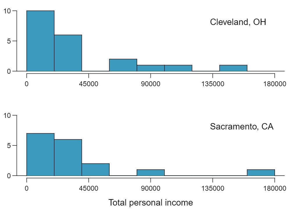
Average income varies from one region of the country to another, and it often reflects both lifestyles and regional living expenses. Suppose a new graduate is considering a job in two locations, Cleveland, OH and Sacramento, CA, and he wants to see whether the average income in one of these cities is higher than the other. He would like to conduct a hypothesis test based on two small samples from the 2000 Census, but he first must consider whether the conditions are met to implement the test. Below are histograms for each city. Should he move forward with the hypothesis test? Explain your reasoning.

26 Oscar winners

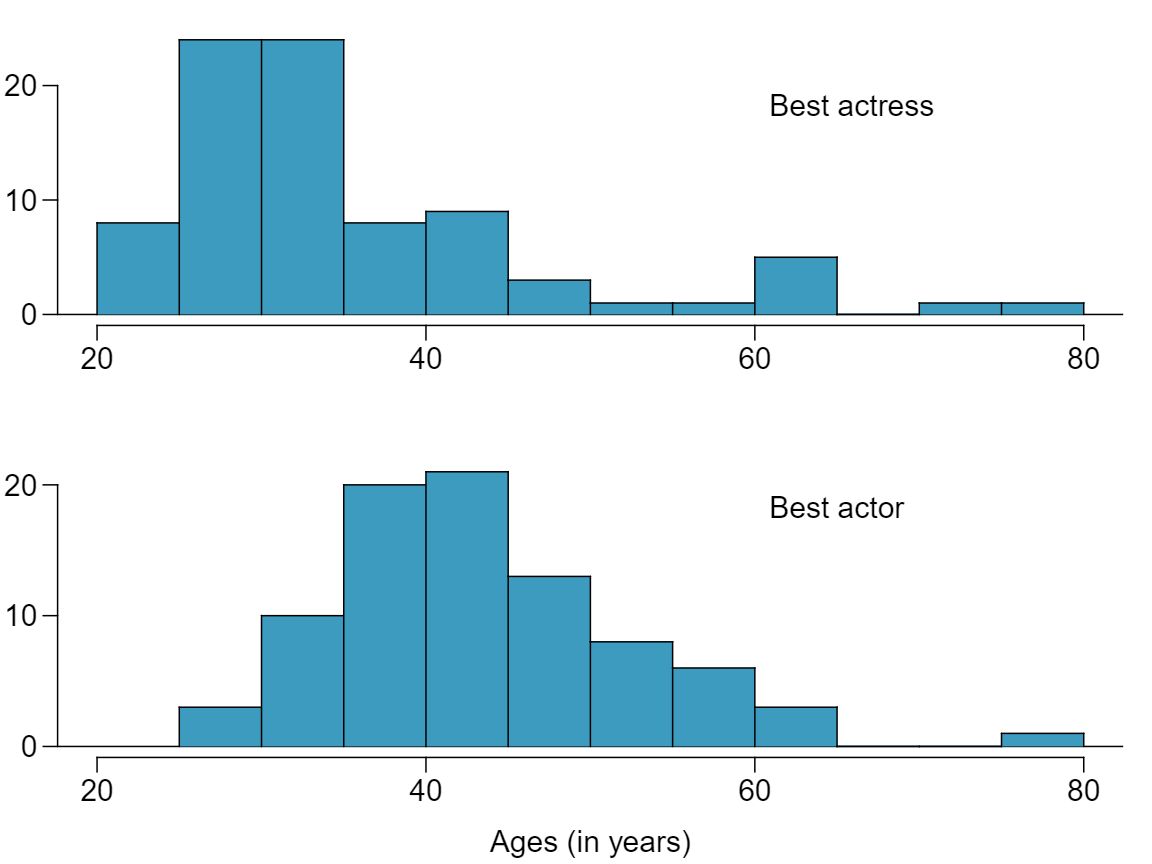
The first Oscar awards for best actor and best actress were given out in 1929. The histograms below show the age distribution for all of the best actor and best actress winners from 1929 to 2012. Summary statistics for these distributions are also provided. Is a hypothesis test appropriate for evaluating whether the difference in the average ages of best actors and actresses might be due to chance? Explain your reasoning. ⁴Oscar winners from 1929-2012, data up to 2009 from the Journal of Statistics Education data archive and for more current data from wikipedia.org/

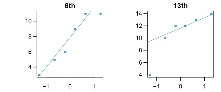
27 Friday the 13\(^{\text{ th } }\text{,}\) Part I.

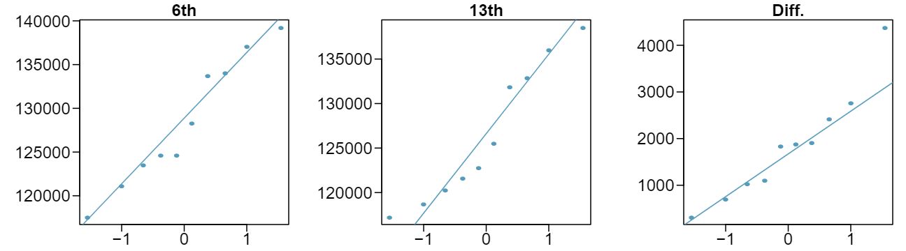
In the early 1990's, researchers in the UK collected data on traffic flow, number of shoppers, and traffic accident related emergency room admissions on Friday the 13\(^{\text{ th } }\) and the previous Friday, Friday the 6\(^{\text{ th } }\text{.}\) The histograms below show the distribution of number of cars passing by a specific intersection on Friday the 6\(^{\text{ th } }\) and Friday the 13\(^{\text{ th } }\) for many such date pairs. Also given are some sample statistics, where the difference is the number of cars on the 6th minus the number of cars on the 13th.⁵T.J. Scanlon et al. “Is Friday the 13th Bad For Your Health?” In: BMJ 307 (1993), pp. 1584-1586

1. Are there any underlying structures in these data that should be considered in an analysis? Explain. Answer

   These data are paired. For example, the Friday the 13th in say, September 1991, would probably be more similar to the Friday the 6th in September 1991 than to Friday the 6th in another month or year.

2. What are the hypotheses for evaluating whether the number of people out on Friday the 6\(^{\text{ th } }\) is different than the number out on Friday the 13\(^{\text{ th } }\text{?}\) Answer

   Let \(\mu_{diff} = \mu_{sixth} - \mu_{thirteenth}\text{.}\) \(H_0: \mu_{diff} = 0\text{.}\) \(H_A: \mu_{diff} \ne 0\text{.}\)

3. Check conditions to carry out the hypothesis test from part (b). Answer

   Independence: The months selected are not random. However, if we think these dates are roughly equivalent to a simple random sample of all such Friday 6th/13th date pairs, then independence is reasonable. To proceed, we must make this strong assumption, though we should note this assumption in any reported results. Normality: With fewer than 10 observations, we would need to use the \(t\) distribution to model the sample mean. The normal probability plot of the differences shows an approximately straight line. There isn't a clear reason why this distribution would be skewed, and since the normal quantile plot looks reasonable, we can mark this condition as reasonably satisfied.

4. Calculate the test statistic and the p-value. Answer

   \(T = 4.94\) for \(df=10-1=9\) \(\to\) p-value \(\lt0.01\text{.}\)

5. What is the conclusion of the hypothesis test? Answer

   Since p-value \(\lt\) 0.05, reject \(H_0\text{.}\) The data provide strong evidence that the average number of cars at the intersection is higher on Friday the 6\(^{\text{th}}\) than on Friday the 13\(^{\text{th}}\text{.}\) (We might believe this intersection is representative of all roads, i.e. there is higher traffic on Friday the 6\(^{\text{th}}\) relative to Friday the 13\(^{\text{th}}\text{.}\) However, we should be cautious of the required assumption for such a generalization.)

6. Interpret the p-value in this context. Answer

   If the average number of cars passing the intersection actually was the same on Friday the 6\(^{\text{th}}\) and \(13^{th}\text{,}\) then the probability that we would observe a test statistic so far from zero is less than 0.01.

7. What type of error might have been made in the conclusion of your test? Explain. Answer

   We might have made a Type 1 error, i.e. incorrectly rejected the null hypothesis.

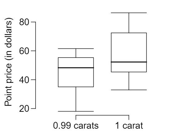
28 Diamonds, Part I

Prices of diamonds are determined by what is known as the 4 Cs: cut, clarity, color, and carat weight. The prices of diamonds go up as the carat weight increases, but the increase is not smooth. For example, the difference between the size of a 0.99 carat diamond and a 1 carat diamond is undetectable to the naked human eye, but the price of a 1 carat diamond tends to be much higher than the price of a 0.99 diamond. In this question we use two random samples of diamonds, 0.99 carats and 1 carat, each sample of size 23, and compare the average prices of the diamonds. In order to be able to compare equivalent units, we first divide the price for each diamond by 100 times its weight in carats. That is, for a 0.99 carat diamond, we divide the price by 99. For a 1 carat diamond, we divide the price by 100. The distributions and some sample statistics are shown below.⁶H. Wickham Deak Link. Spring New York, 2009.

	0.99 carats	1 carat
Mean	$ 44.51	$ 56.81
SD	$ 13.32	$ 16.13
n	23	23

29 Friday the 13\(^{\text{ th } }\text{,}\) Part II.

The Friday the \(13^{th}\) study reported in Exercise 7.5.27 also provides data on traffic accident related emergency room admissions. The distributions of these counts from Friday the 6\(^{\text{ th } }\) and Friday the 13\(^{\text{ th } }\) are shown below for six such paired dates along with summary statistics. You may assume that conditions for inference are met.

	6\(^{\text{ th } }\)	13\(^{\text{ th } }\)	diff
Mean	7.5	10.83	-3.33
SD	3.33	3.6	3.01
n	6	6	6

1. Conduct a hypothesis test to evaluate if there is a difference between the average numbers of traffic accident related emergency room admissions between Friday the 6\(^{\text{ th } }\) and Friday the 13\(^{\text{ th } }\text{.}\) Answer

   \(H_0: \mu_{diff} = 0\text{.}\) \(H_A: \mu_{diff} \ne 0\text{.}\) \(T=-2.71\text{.}\) \(df=5\text{.}\) \(0.02\lt\) p-value \(\lt0.05\text{.}\) Since p-value \(\lt\) 0.05, reject \(H_0\text{.}\) The data provide strong evidence that the average number of traffic accident related emergency room admissions are different between Friday the 6\(^{\text{th}}\) and Friday the 13\(^{\text{th}}\text{.}\) Furthermore, the data indicate that the direction of that difference is that accidents are lower on Friday the \(6^{th}\) relative to Friday the 13\(^{\text{th}}\text{.}\)

2. Calculate a 95% confidence interval for the difference between the average numbers of traffic accident related emergency room admissions between Friday the 6\(^{\text{ th } }\) and Friday the 13\(^{\text{ th } }\text{.}\) Answer

   (-6.49, -0.17).

3. The conclusion of the original study states, “Friday 13th is unlucky for some. The risk of hospital admission as a result of a transport accident may be increased by as much as 52%. Staying at home is recommended.” Do you agree with this statement? Explain your reasoning. Answer

   This is an observational study, not an experiment, so we cannot so easily infer a causal intervention implied by this statement. It is true that there is a difference. However, for example, this does not mean that a responsible adult going out on Friday the \(13^{th}\) has a higher chance of harm than on any other night.

30 Diamonds, Part II

In Exercise 7.5.28, we discussed diamond prices (standardized by weight) for diamonds with weights 0.99 carats and 1 carat. See the table for summary statistics, and then construct a 95% confidence interval for the average difference between the standardized prices of 0.99 and 1 carat diamonds. You may assume the conditions for inference are met.

31 Chicken diet and weight, Part I

Chicken farming is a multi-billion dollar industry, and any methods that increase the growth rate of young chicks can reduce consumer costs while increasing company profits, possibly by millions of dollars. An experiment was conducted to measure and compare the effectiveness of various feed supplements on the growth rate of chickens. Newly hatched chicks were randomly allocated into six groups, and each group was given a different feed supplement. Below are some summary statistics from this data set along with box plots showing the distribution of weights by feed type. ⁷Chicken Weights by Feed Type, from the datasets package in R.

1. Describe the distributions of weights of chickens that were fed linseed and horsebean. Answer

   Chicken fed linseed weighed an average of 218.75 grams while those fed horsebean weighed an average of 160.20 grams. Both distributions are relatively symmetric with no apparent outliers. There is more variability in the weights of chicken fed linseed.

2. Do these data provide strong evidence that the average weights of chickens that were fed linseed and horsebean are different? Use a 5% significance level. Answer

   \(H_0: \mu_{ls} = \mu_{hb}\text{.}\) \(H_A: \mu_{ls} \ne \mu_{hb}\text{.}\) We leave the conditions to you to consider. \(T=3.02\text{,}\) \(df = min(11, 9) = 9\) \(\to\) \(0.01\lt\) p-value \(\lt0.02\text{.}\) Since p-value \(\lt\) 0.05, reject \(H_0\text{.}\) The data provide strong evidence that there is a significant difference between the average weights of chickens that were fed linseed and horsebean.

3. What type of error might we have committed? Explain. Answer

   Type 1, since we rejected \(H_0\text{.}\)

4. Would your conclusion change if we used \(\alpha = 0.01\text{?}\) Answer

   Yes, since p-value \(\gt\) 0.01, we would have failed to reject \(H_0\text{.}\)

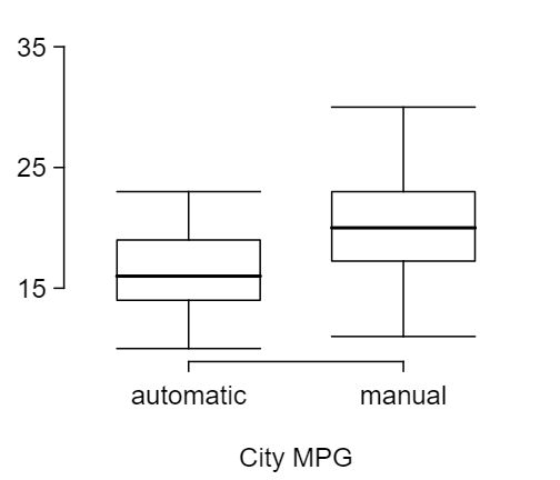
32 Fuel efficiency of manual and automatic cars, Part I

Each year the US Environmental Protection Agency (EPA) releases fuel economy data on cars manufactured in that year. Below are summary statistics on fuel efficiency (in miles/gallon) from random samples of cars with manual and automatic transmissions manufactured in 2012. Do these data provide strong evidence of a difference between the average fuel efficiency of cars with manual and automatic transmissions in terms of their average city mileage? Assume that conditions for inference are satisfied. ⁸U.S. Department of Energy, Fuel Economy Data, 2012 Datafile.

33 Chicken diet and weight, Part II

Casein is a common weight gain supplement for humans. Does it have an effect on chickens? Using data provided in Exercise 7.5.31, test the hypothesis that the average weight of chickens that were fed casein is different than the average weight of chickens that were fed soybean. If your hypothesis test yields a statistically significant result, discuss whether or not the higher average weight of chickens can be attributed to the casein diet. Assume that conditions for inference are satisfied.

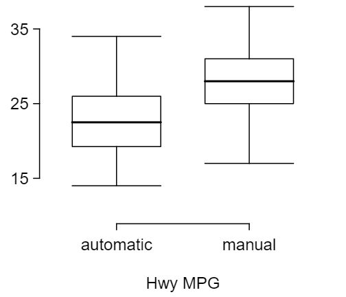
34 Fuel efficiency of manual and automatic cars, Part II

The table provides summary statistics on highway fuel economy of cars manufactured in 2012 (from Exercise 7.5.32). Use these statistics to calculate a 98% confidence interval for the difference between average highway mileage of manual and automatic cars, and interpret this interval in the context of the data.⁹U.S. Department of Energy, Fuel Economy Data, 2012 Datafile.

35 Gaming and distracted eating, Part I

A group of researchers are interested in the possible effects of distracting stimuli during eating, such as an increase or decrease in the amount of food consumption. To test this hypothesis, they monitored food intake for a group of 44 patients who were randomized into two equal groups. The treatment group ate lunch while playing solitaire, and the control group ate lunch without any added distractions. Patients in the treatment group ate 52.1 grams of biscuits, with a standard deviation of 45.1 grams, and patients in the control group ate 27.1 grams of biscuits, with a standard deviation of 26.4 grams. Do these data provide convincing evidence that the average food intake (measured in amount of biscuits consumed) is different for the patients in the treatment group? Assume that conditions for inference are satisfied. ¹⁰R.E. Oldham-Cooper et al. “Playing a computer game during lunch affects fullness, memory for lunch, and later snack intake”. In The Aerican Journal of Clinical Nutrition 93.2 (2011), p. 308.

36 Gaming and distracted eating, Part II

The researchers from Exercise 7.5.35 also investigated the effects of being distracted by a game on how much people eat. The 22 patients in the treatment group who ate their lunch while playing solitaire were asked to do a serial-order recall of the food lunch items they ate. The average number of items recalled by the patients in this group was 4.9, with a standard deviation of 1.8. The average number of items recalled by the patients in the control group (no distraction) was 6.1, with a standard deviation of 1.8. Do these data provide strong evidence that the average number of food items recalled by the patients in the treatment and control groups are different?

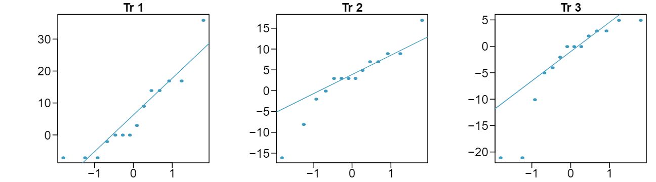
37 Prison isolation experiment, Part I

Subjects from Central Prison in Raleigh, NC, volunteered for an experiment involving an “isolation” experience. The goal of the experiment was to find a treatment that reduces subjects' psychopathic deviant \(T\)-scores. This score measures a person's need for control or their rebellion against control, and it is part of a commonly used mental health test called the Minnesota Multiphasic Personality Inventory (MMPI) test. The experiment had three treatment groups:

1. Four hours of sensory restriction plus a 15 minute “therapeutic” tape advising that professional help is available.
2. Four hours of sensory restriction plus a 15 minute “emotionally neutral” tape on training hunting dogs.
3. Four hours of sensory restriction but no taped message.

Forty-two subjects were randomly assigned to these treatment groups, and an MMPI test was administered before and after the treatment. Distributions of the differences between pre and post treatment scores (pre - post) are shown below, along with some sample statistics. Use this information to independently test the effectiveness of each treatment. Make sure to clearly state your hypotheses, check conditions, and interpret results in the context of the data.¹¹Prison isolation experiment

38 True / False: comparing means

Determine if the following statements are true or false, and explain your reasoning for statements you identify as false.

1. When comparing means of two samples where \(n_1 = 20\) and \(n_2 = 40\text{,}\) we can use the normal model for the difference in means since \(n_2 \ge 30\text{.}\)

2. As the degrees of freedom increases, the \(t\)-distribution approaches normality.

3. We use a pooled standard error for calculating the standard error of the difference between means when sample sizes of groups are equal to each other.

39 Fill in the blank

When doing an ANOVA, you observe large differences in means between groups. Within the ANOVA framework, this would most likely be interpreted as evidence strongly favoring the __________ hypothesis.

40 Which test?

We would like to test if students who are in the social sciences, natural sciences, arts and humanities, and other fields spend the same amount of time studying for this course. What type of test should we use? Explain your reasoning.

41 Chicken diet and weight, Part III

In Exercise 7.5.31 and Exercise 7.5.33 we compared the effects of two types of feed at a time. A better analysis would first consider all feed types at once: casein, horsebean, linseed, meat meal, soybean, and sunflower. The ANOVA output below can be used to test for differences between the average weights of chicks on different diets.

Conduct a hypothesis test to determine if these data provide convincing evidence that the average weight of chicks varies across some (or all) groups. Make sure to check relevant conditions. Figures and summary statistics are shown below.

42 Teaching descriptive statistics

A study compared five different methods for teaching descriptive statistics. The five methods were traditional lecture and discussion, programmed textbook instruction, programmed text with lectures, computer instruction, and computer instruction with lectures. 45 students were randomly assigned, 9 to each method. After completing the course, students took a 1-hour exam.

1. What are the hypotheses for evaluating if the average test scores are different for the different teaching methods?

2. What are the degrees of freedom associated with the \(F\)-test for evaluating these hypotheses?

3. Suppose the p-value for this test is 0.0168. What is the conclusion?

43 Coffee, depression, and physical activity

Caffeine is the world's most widely used stimulant, with approximately 80% consumed in the form of coffee. Participants in a study investigating the relationship between coffee consumption and exercise were asked to report the number of hours they spent per week on moderate (e.g., brisk walking) and vigorous (e.g., strenuous sports and jogging) exercise. Based on these data the researchers estimated the total hours of metabolic equivalent tasks (MET) per week, a value always greater than 0. The table below gives summary statistics of MET for women in this study based on the amount of coffee consumed.¹²M. Lucas et al. “(LINK ISSUE) Coffee, caffeine, and risk of depression among women”. In: Archives of internal medicine 171.17 (2011), p. 1571.

1. Write the hypotheses for evaluating if the average physical activity level varies among the different levels of coffee consumption. Answer

   \(H_0\text{:}\) The population mean of MET for each group is equal to the others. \(H_A\text{:}\) At least one pair of means is different.

2. Check conditions and describe any assumptions you must make to proceed with the test. Answer

   Independence: We don't have any information on how the data were collected, so we cannot assess independence. To proceed, we must assume the subjects in each group are independent. In practice, we would inquire for more details. Approx. normal: The data are bound below by zero and the standard deviations are larger than the means, indicating very strong strong skew. However, since the sample sizes are extremely large, even extreme skew is acceptable. Constant variance: This condition is sufficiently met, as the standard deviations are reasonably consistent across groups.

3. Below is part of the output associated with this test. Fill in the empty cells.

   	Df	Sum Sq	Mean Sq	F value	Pr(\(\gt\)F)
   coffee					0.0003
   Residuals		25,564,819
   Total		25,575,327

   Answer

   See below, with the last column omitted:

   	Df	Sum Sq	Mean Sq	F value
   coffee	4	10508	2627	5.2
   Residuals	50734	25564819	504
   Total	50738	25575327

4. What is the conclusion of the test? Answer

   Since p-value is very small, reject \(H_0\text{.}\) The data provide convincing evidence that the average MET differs between at least one pair of groups.

44 Student performance across discussion sections

A professor who teaches a large introductory statistics class (197 students) with eight discussion sections would like to test if student performance differs by discussion section, where each discussion section has a different teaching assistant. The summary table below shows the average final exam score for each discussion section as well as the standard deviation of scores and the number of students in each section.

The ANOVA output below can be used to test for differences between the average scores from the different discussion sections.

Conduct a hypothesis test to determine if these data provide convincing evidence that the average score varies across some (or all) groups. Check conditions and describe any assumptions you must make to proceed with the test.

45 GPA and major

Undergraduate students taking an introductory statistics course at Duke University conducted a survey about GPA and major. The side-by-side box plots show the distribution of GPA among three groups of majors. Also provided is the ANOVA output.

1. Write the hypotheses for testing for a difference between average GPA across majors. Answer

   \(H_0\text{:}\) Average GPA is the same for all majors. \(H_A\text{:}\) At least one pair of means are different.

2. What is the conclusion of the hypothesis test? Answer

   Since p-value \(\gt\) 0.05, fail to reject \(H_0\text{.}\) The data do not provide convincing evidence of a difference between the average GPAs across three groups of majors.

3. How many students answered these questions on the survey, i.e. what is the sample size? Answer

   The total degrees of freedom is \(195 + 2 = 197\text{,}\) so the sample size is \(197+1=198\text{.}\)

46 Work hours and education

The General Social Survey collects data on demographics, education, and work, among many other characteristics of US residents. ¹³National Opinion Research Center, General Social Survey 2010. Using ANOVA, we can consider educational attainment levels for all 1,172 respondents at once. Below are the distributions of hours worked by educational attainment and relevant summary statistics that will be helpful in carrying out this analysis.

1. Write hypotheses for evaluating whether the average number of hours worked varies across the five groups.

2. Check conditions and describe any assumptions you must make to proceed with the test.

3. Below is part of the output associated with this test. Fill in the empty cells.

   	Df	Sum Sq	Mean Sq	F value	Pr(\(\gt\)F)
   degree			501.54		0.0682
   Residuals		267,382
   Total

4. What is the conclusion of the test?

47 True / False: ANOVA, Part I

Determine if the following statements are true or false in ANOVA, and explain your reasoning for statements you identify as false.

1. As the number of groups increases, the modified significance level for pairwise tests increases as well. Answer

   False. As the number of groups increases, so does the number of comparisons and hence the modified significance level decreases.

2. As the total sample size increases, the degrees of freedom for the residuals increases as well. Answer

   True.

3. The constant variance condition can be somewhat relaxed when the sample sizes are relatively consistent across groups. Answer

   True.

4. The independence assumption can be relaxed when the total sample size is large. Answer

   False. We need observations to be independent regardless of sample size.

48 Child care hours

The China Health and Nutrition Survey aims to examine the effects of the health, nutrition, and family planning policies and programs implemented by national and local governments.¹⁴UNC Carolina Population Center, China Health and Nutrition Survey, 2006 It, for example, collects information on number of hours Chinese parents spend taking care of their children under age 6. The side-by-side box plots below show the distribution of this variable by educational attainment of the parent. Also provided below is the ANOVA output for comparing average hours across educational attainment categories.

1. Write the hypotheses for testing for a difference between the average number of hours spent on child care across educational attainment levels.

2. What is the conclusion of the hypothesis test?

49 Prison isolation experiment, Part II

Exercise 7.5.37 introduced an experiment that was conducted with the goal of identifying a treatment that reduces subjects' psychopathic deviant \(T\)-scores, where this score measures a person's need for control or his rebellion against control. In Exercise 7.5.37 you evaluated the success of each treatment individually. An alternative analysis involves comparing the success of treatments. The relevant ANOVA output is given below.

1. What are the hypotheses? Answer

   \(H_0\text{:}\) Average score difference is the same for all treatments. \(H_A\text{:}\) At least one pair of means are different.

2. What is the conclusion of the test? Use a 5% significance level. Answer

   We should check conditions. If we look back to the earlier exercise, we will see that the patients were randomized, so independence is satisfied. There are some minor concerns about skew, especially with the third group, though this may be acceptable. The standard deviations across the groups are reasonably similar. Since the p-value is less than 0.05, reject \(H_0\text{.}\) The data provide convincing evidence of a difference between the average reduction in score among treatments.

3. If in part (b) you determined that the test is significant, conduct pairwise tests to determine which groups are different from each other. If you did not reject the null hypothesis in part (b), recheck your solution. Answer

   We determined that at least two means are different in part (b), so we now conduct \(K=3\times2/2=3\) pairwise \(t\)-tests that each use \(\alpha=0.05/3 = 0.0167\) for a significance level. Use the following hypotheses for each pairwise test. \(H_0\text{:}\) The two means are equal. \(H_A\text{:}\) The two means are different. The sample sizes are equal and we use the pooled SD, so we can compute \(SE=3.7\) with the pooled \(df=39\text{.}\) The p-value only for Trmt 1 vs. Trmt 3 may be statistically significant: \(0.01\lt\) p-value \(\lt0.02\text{.}\) Since we cannot tell, we should use a computer to get the p-value, 0.015, which is statistically significant for the adjusted significance level. That is, we have identified Treatment 1 and Treatment 3 as having different effects. Checking the other two comparisons, the differences are not statistically significant.

50 True / False: ANOVA, Part II

Determine if the following statements are true or false, and explain your reasoning for statements you identify as false.

If the null hypothesis that the means of four groups are all the same is rejected using ANOVA at a 5% significance level, then ...

1. we can then conclude that all the means are different from one another.

2. the standardized variability between groups is higher than the standardized variability within groups.

3. the pairwise analysis will identify at least one pair of means that are significantly different.

4. the appropriate \(\alpha\) to be used in pairwise comparisons is 0.05 / 4 = 0.0125 since there are four groups.