Chapter 8 Introduction to linear regression
¶Linear regression is a very powerful statistical technique. Many people have some familiarity with regression just from reading the news, where graphs with straight lines are overlaid on scatterplots. Linear models can be used for prediction or to evaluate whether there is a linear relationship between two numerical variables.
Figure 8.0.1 shows two variables whose relationship can be modeled perfectly with a straight line. The equation for the line is
Imagine what a perfect linear relationship would mean: you would know the exact value of \(y\) just by knowing the value of \(x\text{.}\) This is unrealistic in almost any natural process. For example, if we took family income \(x\text{,}\) this value would provide some useful information about how much financial support \(y\) a college may offer a prospective student. However, there would still be variability in financial support, even when comparing students whose families have similar financial backgrounds.
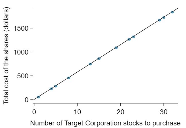
TGT, April 26th, 2012), and the total cost of the shares were reported. Because the cost is computed using a linear formula, the linear fit is perfect.Linear regression assumes that the relationship between two variables, \(x\) and \(y\text{,}\) can be modeled by a straight line:
1 \(\beta_0, \beta_1\) Linear model parameterswhere \(\beta_0\) and \(\beta_1\) represent two model parameters (\(\beta\) is the Greek letter beta). (This use of \(\beta\) has nothing to do with the \(\beta\) we used to describe the probability of a Type 2 Error.) These parameters are estimated using data, and we write their point estimates as \(b_0\) and \(b_1\text{.}\) When we use \(x\) to predict \(y\text{,}\) we usually call \(x\) the explanatory or predictor variable, and we call \(y\) the response.
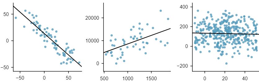
It is rare for all of the data to fall on a straight line, as seen in the three scatterplots in Figure 8.0.2. In each case, the data fall around a straight line, even if none of the observations fall exactly on the line. The first plot shows a relatively strong downward linear trend, where the reidxing variability in the data around the line is minor relative to the strength of the relationship between \(x\) and \(y\text{.}\) The second plot shows an upward trend that, while evident, is not as strong as the first. The last plot shows a very weak downward trend in the data, so slight we can hardly notice it. In each of these examples, we will have some uncertainty regarding our estimates of the model parameters, \(\beta_0\) and \(\beta_1\text{.}\) For instance, we might wonder, should we move the line up or down a little, or should we tilt it more or less? As we move forward in this chapter, we will learn different criteria for line-fitting, and we will also learn about the uncertainty associated with estimates of model parameters.
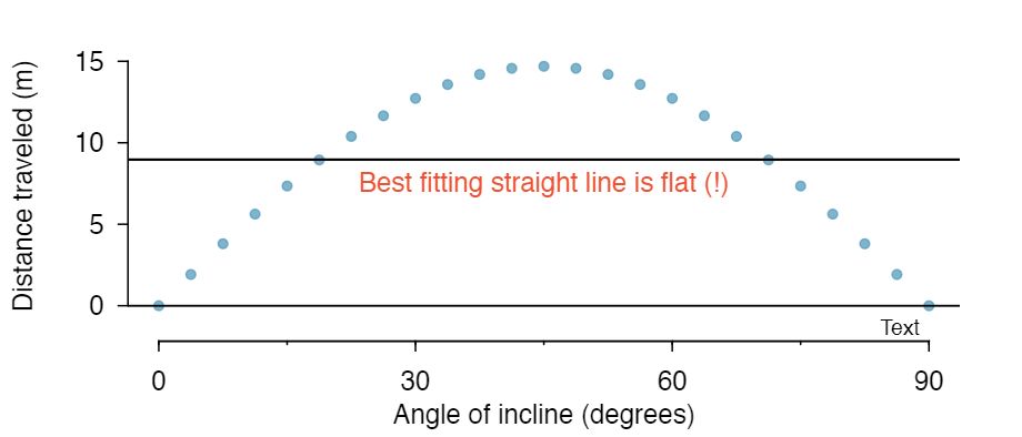
We will also see examples in this chapter where fitting a straight line to the data, even if there is a clear relationship between the variables, is not helpful. One such case is shown in Figure 8.0.3 where there is a very strong relationship between the variables even though the trend is not linear. We will discuss nonlinear trends in this chapter and the next, but the details of fitting nonlinear models are saved for a later course.