
Section 1.2 Data basics
¶Effective presentation and description of data is a first step in most analyses. This section introduces one structure for organizing data as well as some terminology that will be used throughout this book.
OpenIntro: Data basics video
Subsection 1.2.1 Observations, variables, and data matrices
Table 1.2.2 displays rows 1, 2, 3, and 50 of a data set concerning 50 emails received during early 2012. These observations will be referred to as the email50 data set, and they are a random sample from a larger data set that we will see in Section 2.3.
Each row in the table represents a single email or case. 1 A case is also sometimes called a unit of observation or an observational unit. The columns represent characteristics, called variables, for each of the emails. For example, the first row represents email 1, which is not spam, contains 21,705 characters, 551 line breaks, is written in HTML format, and contains only small numbers.
In practice, it is especially important to ask clarifying questions to ensure important aspects of the data are understood. For instance, it is always important to be sure we know what each variable means and the units of measurement. Descriptions of all five email variables are given in Table 1.2.3.
spam |
num_char |
line_breaks |
format |
number |
|
| 1 | no | 21,705 | 551 | html | small |
| 2 | no | 7,011 | 183 | html | big |
| 3 | yes | 631 | 28 | text | none |
| \(\vdots\) | \(\vdots\) | \(\vdots\) | \(\vdots\) | \(\vdots\) | \(\vdots\) |
| 50 | no | 15,829 | 242 | html | small |
email50 data matrix.| variable | description |
spam |
Specifies whether the message was spam |
num_char |
The number of characters in the email |
line_breaks |
The number of line breaks in the email (not including text wrapping) |
format |
Indicates if the email contained special formatting, such as bolding, tables, or links, which would indicate the message is in HTML format |
number |
Indicates whether the email contained no number, a small number (under 1 million), or a large number |
email50 data set.The data in Table 1.2.2 represent a data matrix, which is a common way to organize data. Each row of a data matrix corresponds to a unique case, and each column corresponds to a variable. A data matrix for the stroke study introduced in Section 1.1 is shown in Table 1.1.2, where the cases were patients and there were three variables recorded for each patient.
Data matrices are a convenient way to record and store data. If another individual or case is added to the data set, an additional row can be easily added. Similarly, another column can be added for a new variable.
We consider a publicly available data set that summarizes information about the 3,143 counties in the United States, and we call this the county data set. This data set includes information about each county: its name, the state where it resides, its population in 2000 and 2010, per capita federal spending, poverty rate, and five additional characteristics. How might these data be organized in a data matrix? Reminder: look in the footnotes for answers to in-text exercises. 2 Each county may be viewed as a case, and there are eleven pieces of information recorded for each case. A table with 3,143 rows and 11 columns could hold these data, where each row represents a county and each column represents a particular piece of information.
Seven rows of the county data set are shown in Table 1.2.6, and the variables are summarized in Table 1.2.7. These data were collected from the US Census website. 3 www.quickfacts.census.gov/qfd/index.html
Subsection 1.2.2 Types of variables
¶Examine the fed_spend, pop2010, state, and smoking_ban variables in the county data set. Each of these variables is inherently different from the other three yet many of them share certain characteristics.
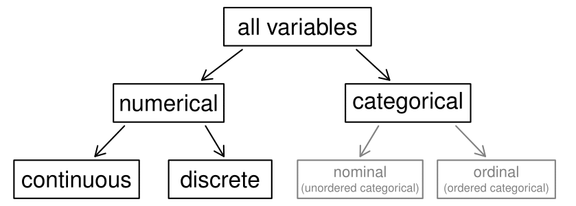
First consider fed_spend, which is said to be a numerical variable since it can take a wide range of numerical values, and it is sensible to add, subtract, or take averages with those values. On the other hand, we would not classify a variable reporting telephone area codes as numerical since their average, sum, and difference have no clear meaning.
The pop2010 variable is also numerical, although it seems to be a little different than fed_spend. This variable of the population count can only take whole non-negative numbers (0, 1, 2, ...). For this reason, the population variable is said to be discrete since it can only take numerical values with jumps. On the other hand, the federal spending variable is said to be continuous.
The variable state can take up to 51 values after accounting for Washington, DC: AL, ..., and WY. Because the responses themselves are categories, state is called a categorical variable, 4 Sometimes also called a nominal variable. and the possible values are called the variable's levels.
Finally, consider the smoking_ban variable, which describes the type of county-wide smoking ban and takes values none, partial, or comprehensive in each county. This variable seems to be a hybrid: it is a categorical variable but the levels have a natural ordering. A variable with these properties is called an ordinal variable. To simplify analyses, any ordinal variables in this book will be treated as categorical variables.
name |
state |
pop2000 |
pop2010 |
fed_spend |
poverty |
homeownership |
multiunit |
income |
med_income |
smoking_ban |
|
| 1 | Autauga | AL | 43671 | 54571 | 6.068 | 10.6 | 77.5 | 7.2 | 24568 | 53255 | none |
| 2 | Baldwin | AL | 140415 | 182265 | 6.140 | 12.2 | 76.7 | 22.6 | 26469 | 50147 | none |
| 3 | Barbour | AL | 29038 | 27457 | 8.752 | 25.0 | 68.0 | 11.1 | 15875 | 33219 | none |
| 4 | Bibb | AL | 20826 | 22915 | 7.122 | 12.6 | 82.9 | 6.6 | 19918 | 41770 | none |
| 5 | Blount | AL | 51024 | 57322 | 5.131 | 13.4 | 82.0 | 3.7 | 21070 | 45549 | none |
| \(\vdots\) | \(\vdots\) | \(\vdots\) | \(\vdots\) | \(\vdots\) | \(\vdots\) | \(\vdots\) | \(\vdots\) | \(\vdots\) | \(\vdots\) | \(\vdots\) | \(\vdots\) |
| 3142 | Washakie | WY | 8289 | 8533 | 8.714 | 5.6 | 70.9 | 10.0 | 28557 | 48379 | none |
| 3143 | Weston | WY | 6644 | 7208 | 6.695 | 7.9 | 77.9 | 6.5 | 28463 | 53853 | none |
county data set.| variable | description |
name |
County name |
state |
State where the county resides (also including the District of Columbia) |
pop2000 |
Population in 2000 |
pop2010 |
Population in 2010 |
fed_spend |
Federal spending per capita |
poverty |
Percent of the population in poverty |
homeownership |
Percent of the population that lives in their own home or lives with the owner (e.g. children living with parents who own the home) |
multiunit |
Percent of living units that are in multi-unit structures (e.g. apartments) |
income |
Income per capita |
med_income |
Median household income for the county, where a household's income equals the total income of its occupants who are 15 years or older |
smoking_ban |
Type of county-wide smoking ban in place at the end of 2011, which takes one of three values: none, partial, or comprehensive, where a comprehensive ban means smoking was not permitted in restaurants, bars, or workplaces, and partial means smoking was banned in at least one of those three locations |
county data set.Example 1.2.8
Data were collected about students in a statistics course. Three variables were recorded for each student: number of siblings, student height, and whether the student had previously taken a statistics course. Classify each of the variables as continuous numerical, discrete numerical, or categorical.
Solution
The number of siblings and student height represent numerical variables. Because the number of siblings is a count, it is discrete. Height varies continuously, so it is a continuous numerical variable. The last variable classifies students into two categories — those who have and those who have not taken a statistics course — which makes this variable categorical.
Guided Practice 1.2.9
Consider the variables group and outcome (at 30 days) from the stent study in Section 1.1. Are these numerical or categorical variables? 5 There are only two possible values for each variable, and in both cases they describe categories. Thus, each is a categorical variable.
Subsection 1.2.3 Relationships between variables
¶Many analyses are motivated by a researcher looking for a relationship between two or more variables. A social scientist may like to answer some of the following questions:
Is federal spending, on average, higher or lower in counties with high rates of poverty?
If homeownership is lower than the national average in one county, will the percent of multi-unit structures in that county likely be above or below the national average?
Which counties have a higher average income: those that enact one or more smoking bans or those that do not?
To answer these questions, data must be collected, such as the county data set shown in Table 1.2.6. Examining summary statistics could provide insights for each of the three questions about counties. Additionally, graphs can be used to visually summarize data and are useful for answering such questions as well.
Scatterplots are one type of graph used to study the relationship between two numerical variables. Figure 1.2.11 compares the variables fed_spend and poverty. Each point on the plot represents a single county. For instance, the highlighted dot corresponds to County 1088 in the county data set: Owsley County, Kentucky, which had a poverty rate of 41.5% and federal spending of $21.50 per capita. The scatterplot suggests a relationship between the two variables: counties with a high poverty rate also tend to have slightly more federal spending. We might brainstorm as to why this relationship exists and investigate each idea to determine which is the most reasonable explanation.
Guided Practice 1.2.10
Examine the variables in the email50 data set, which are described in Table 1.2.3. Create two questions about the relationships between these variables that are of interest to you. 6 Two sample questions: (1) Intuition suggests that if there are many line breaks in an email then there would also tend to be many characters: does this hold true? (2) Is there a connection between whether an email format is plain text (versus HTML) and whether it is a spam message?
The fed_spend and poverty variables are said to be associated because the plot shows a discernible pattern. When two variables show some connection with one another, they are called associated variables. Associated variables can also be called dependent variables and vice-versa.
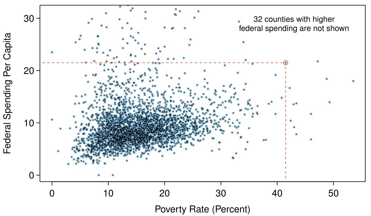
fed_spend against poverty . Owsley County of Kentucky, with a poverty rate of 41.5%and federal spending $21.50 per capita, is highlightedExample 1.2.12
The relationship between the homeownership rate and the percent of units in multi-unit structures (e.g. apartments, condos) is visualized using a scatterplot in Figure 1.2.13. Are these variables associated?
Solution
It appears that the larger the fraction of units in multi-unit structures, the lower the homeownership rate. Since there is some relationship between the variables, they are associated.
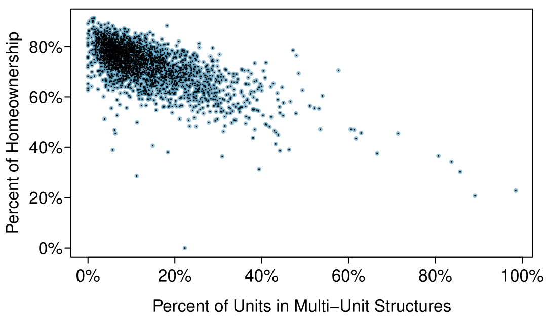
Because there is a downward trend in Figure 1.2.13 — counties with more units in multi-unit structures are associated with lower homeownership — these variables are said to be negatively associated. A positive association is shown in the relationship between the poverty and fed_spend variables represented in Figure 1.2.11, where counties with higher poverty rates tend to receive more federal spending per capita.
If two variables are not associated, then they are said to be independent. That is, two variables are independent if there is no evident relationship between the two.
Associated or independent, not both
A pair of variables are either related in some way (associated) or not (independent). No pair of variables is both associated and independent.