
Paired data
Two sets of observations are paired if each observation in one set has a special correspondence or connection with exactly one observation in the other data set.
Are textbooks actually cheaper online? Here we compare the price of textbooks at UCLA's bookstore and prices at Amazon.com. Seventy-three UCLA courses were randomly sampled in Spring 2010, representing less than 10% of all UCLA courses. 1 When a class had multiple books, only the most expensive text was considered. A portion of this data set is shown in Table 7.2.2.
| dept | course | ucla | amazon | diff | |
| 1 | Am Ind | C170 | 27.67 | 27.95 | -0.28 |
| 2 | Anthro | 9 | 40.59 | 31.14 | 9.45 |
| 3 | Anthro | 135T | 31.68 | 32.00 | -0.32 |
| 4 | Anthro | 191HB | 16.00 | 11.52 | 4.48 |
| \(\vdots\) | \(\vdots\) | \(\vdots\) | \(\vdots\) | \(\vdots\) | \(\vdots\) |
| 72 | Wom Std | M144 | 23.76 | 18.72 | 5.04 |
| 73 | Wom Std | 285 | 27.70 | 18.22 | 9.48 |
textbooks data set.Each textbook has two corresponding prices in the data set: one for the UCLA bookstore and one for Amazon. Therefore, each textbook price from the UCLA bookstore has a natural correspondence with a textbook price from Amazon. When two sets of observations have this special correspondence, they are said to be paired.
Two sets of observations are paired if each observation in one set has a special correspondence or connection with exactly one observation in the other data set.
To analyze paired data, it is often useful to look at the difference in outcomes of each pair of observations. In the textbook data set, we look at the difference in prices, which is represented as the diff variable in the textbooks data. Here the differences are taken as
for each book. It is important that we always subtract using a consistent order; here Amazon prices are always subtracted from UCLA prices. If this difference is positive, the UCLA price is higher. If ths difference is negative, the Amazon price is higher. If this difference is zero, the two prices are equal. A histogram of these differences is shown in Figure 7.2.3. Using differences between paired observations is a common and useful way to analyze paired data.
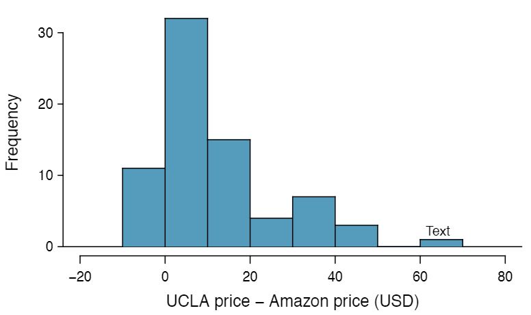
The first difference shown in Table 7.2.2 is computed as \(27.67-27.95=-0.28\text{.}\) Based on the table and on the histogram of differences in Figure 7.2.3, which store tends to have the higher prices in the sample? 2 Because the most of the differences are positive, UCLA prices tend to be higher than Amazon. Note that it is important to identify the order in which the differences are taken.
To analyze a paired data set, we use the exact same tools that we developed in the previous section. Now we apply them to the differences in the paired observations.
| \(n_{_{diff}}\) | \(\bar{x}_{_{diff}}\) | \(s_{_{diff}}\) | ||
| 73 | 12.76 | 14.26 | ||
Set up and implement a hypothesis test to determine whether, on average, there is a difference between Amazon's price for a book and the UCLA bookstore's price.
There are two scenarios: there is no difference or there is some difference in average prices. The no difference scenario is always the null hypothesis:
\(\mu_{diff}=0\text{.}\) There is no difference in the average textbook price.
\(\mu_{diff} \neq 0\text{.}\) There is a difference in average prices.
The standard deviation of all of the differences in unknown, so we will use the standard deviation of the sample differences. The observations are based on a simple random sample from less than 10% of all books sold at the bookstore, so independence is reasonable; the distribution of differences, shown in Figure 7.2.3, is strongly skewed, but the sample size \(n=73\) is well over 30. Because all three conditions are reasonably satisfied, we can conclude the \(t\)-test is reasonable.
We compute the standard error associated with \(\bar{x}_{diff}\) using the standard deviation of the differences (\(s_{_{diff}}=14.26\)) and the number of differences (\(n_{_{diff}}=73\)):
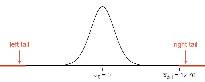
To visualize the p-value, the sampling distribution of \(\bar{x}_{diff}\) is drawn as though \(H_0\) is true, which is shown in Figure 7.2.7. The p-value is represented by the two (very) small tails.
To find the tail areas, we compute the test statistic, which is the \(T\) score of \(\bar{x}_{diff}\) under the null condition that the actual mean difference is 0:
This \(T\) score is so large it isn't even in the table, which ensures the single tail area will be 0.0002 or smaller. A calculator gives a tail area as \(4.5\times 10^{-11}\text{.}\) Since the p-value corresponds to both tails in this case and the \(t\)-distribution is symmetric, the p-value can be estimated as twice the one-tail area:
Because the p-value is less than 0.05, we reject the null hypothesis. We have found convincing evidence that Amazon is, on average, cheaper than the UCLA bookstore for UCLA course textbooks.
State the name of the test being used.
Matched pairs \(t\)-test.
Verify conditions.
Paired data from a random sample or experiment.
Population of differences is known to be normal OR \(n_{diff}\ge 30\) OR graph of sample differences is approximately symmetric with no outliers, making the assumption that population of differences is normal a reasonable one.
Write the hypotheses in plain language, then set them up in mathematical notation.
H\(_0: \mu_{diff}=0\)
H\(_0: \mu_{diff} \ne \text{ or } \lt \text{ or } > 0\)
Identify the significance level \(\alpha\text{.}\)
Calculate the test statistic and \(df\text{:}\) \(\text{t} = \frac{\text{ point estimate } - \text{ null value } }{\text{ SE of estimate } }\)
The point estimate is \(\bar{x}_{diff}\)
Use \(SE = \frac{s_{diff}}{\sqrt{n_{diff}}}\)
\(df=n_{diff}-1\)
Find the p-value and compare it to \(\alpha\) to determine whether to reject or not reject \(H_0\text{.}\)
Write the conclusion in the context of the question.
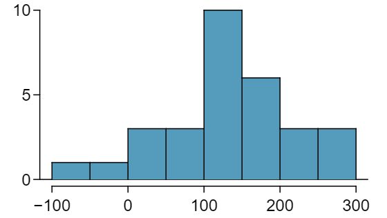
An SAT preparation company claims that its students' scores improve by over 100 points on average after their course. A consumer group would like to evaluate this claim, and they collect data on a random sample of 30 students who took the class. Each of these students took the SAT before and after taking the company's course, and so we have a difference in scores for each student. We will examine these differences \(x_1=57\text{,}\) \(x_2=133\text{,}\) ..., \(x_{30}=140\) as a sample to evaluate the company's claim. The distribution of the differences, shown in Figure 7.2.8, has mean 135.9 and standard deviation 82.2. Do these data provide convincing evidence to back up the company's claim? 3 These are paired data, so we analyze the score differences with a matched pairs \(t\)-test. Conditions: This is a random sample from less than 10% of the company's students (assuming they have more than 300 former students), so the independence condition is reasonable. \(n=30\ge 30\text{.}\) This is a one-sided test. \(H_0\text{:}\) student scores do not improve by more than 100 after taking the company's course. \(\mu_{_{diff}} = 100\) \(H_A\text{:}\) students scores improve by more than 100 points on average after taking the company's course. \(\mu_{_{diff}} \gt 100\text{.}\) Let
\begin{align*}
\amp \amp \alpha=0.05 \amp \amp SE_{diff} = \frac{82.2}{\sqrt{30}} = 15.0\\
\amp \amp T = \frac{135.9-100}{15.0}=2.4 \amp \text { with } df=29
\end{align*}
p-value\(=0.012\lt \alpha\) so we reject the null hypothesis. The data provide convincing evidence to support the company's claim that student scores improve by more than 100 points following the class.
Because we rejected the null hypothesis, does this mean that taking the company's class improves student scores by more than 100 points on average? 4 This is an observational study, so we cannot make this causal conclusion. For instance, maybe SAT test takers tend to improve their score over time even if they don't take a special SAT class, or perhaps only the most motivated students take such SAT courses.
In the previous examples, we carried out a matched pairs \(t\)-test, where the null hypothesis was that the true average of the paired differences is zero. Sometimes we want to estimate the true average of paired differences with a confidence interval, and we use a matched pairs \(t\)-interval. Consider again the table of data on the difference in price between UCLA and Amazon for each of the 73 books sampled.
| \(n_{_{diff}}\) | \(\bar{x}_{_{diff}}\) | \(s_{_{diff}}\) | ||
| 73 | 12.76 | 14.26 | ||
We we construct a 95% confidence interval for the average price difference between books at the UCLA bookstore and books on Amazon. Conditions have already verified and the standard error computed in Example 7.2.6. To find the interval, identify \(t ^{\star}\text{.}\) Since \(df = 72\) is not on the \(t\)-table, round the \(df\) down to 60 to get a \(t^{\star}\) of 2.00 for 95% confidence. Plugging in the \(t^{\star}\text{,}\) the point estimate, and the standard error into the confidence interval formula we get:
We are 95% confident that the UCLA bookstore is, on average, between $9.42 and $16.10 more expensive than Amazon for UCLA course books. This interval does not contain zero, so it is consistent with the fact that our earlier hypothesis test rejected the null hypothesis that the average difference was 0. Because our interval is entirely above 0, we have evidence that the true average difference is not 0. Unlike the test of hypothesis, though, the confidence interval tells us about how much more expensive the UCLA bookstore is.
State the name of the CI being used.
Matched pairs \(t\)-interval
Verify conditions.
Paired data from a random sample or experiment.
Population of diferrences is known to be normal OR \(n_{diff}\ge 30\) OR graph of sample differences is approximately symmetric with no outliers, making the assumption that the population of differences is normal a reasonable one.
Plug in the numbers and write the interval in the form
The point estimate of \(\bar{x}_{diff}\)
\(df=n_{diff}-1\)
Plug in the critical value \(t^\star\) using the \(t\)-table at row \(n_{diff}-1\)
Use \(SE = \frac{s_{diff}}{\sqrt{n_{diff}}}\)
Evaluate the CI and write in the form ( \(\_\) , \(\_\) ).
Interpret the interval: “We are [XX]% confident that the true mean of the differences in [...] is between [...] and [...].”
State the conclusion to the original question.
In the SAT preparation company example, we saw that \(\bar{x}_{diff}\) was 135.9 and \(s_{diff}\) was 82.2. That is, the average change in students' scores after the class was a 135.9 point increase and the SD of the change or difference in their scores was 82.2 points. Construct a 95% confidence interval to estimate the true average change in score after taking the class. Is there evidence for the company's claim that students score an average of 100 points higher after the class? 5 Because this is a before and after scenario, we use a matched pairs \(t\)-interval. The conditions were verified in the previous section. The confidence interval is : \(135.9\ \pm 2.045(15.0) \to (105.2, 166.6)\text{.}\) We can be 95% confident that the true average increase in scores after the prep class is between 105.2 and 166.6. Because the entire interval is above 100, there is evidence that on average students score more than 100 points higher after the course. Recall that this does not prove that the increase is due to the course.
The 95% confidence interval in the previous exercise was calculated as (105.2, 166.6). True or false: about 95% of the students that take the class saw an increase of at least 105.2 points. 6 False. This confidence interval estimates the average increase - not the increase of individuals. As can be seen in Figure 7.2.8, much greater than 5% saw an increase of less than 105.2 points. Some individuals even saw a decrease in their score as indicated by the negative differences.
The matched pairs \(t\)-test and CI proceed the same way as the 1-sample \(t\)-test and confidence interval. Instead of using the data or the summary statistics from the single sample, make sure to use the data of differences or the summary statistics for the differences.
Use STAT, TESTS, T-Test.
Choose STAT.
Right arrow to TESTS.
Down arrow and choose 2:T-Test.
Choose Data if you have all the data or Stats if you have the mean and standard deviation.
Let \(\mu_0\) be the null or hypothesized value of \(\mu_{diff}\text{.}\)
If you choose Data, let List be L3 or the list in which you entered the differences (don't forget to enter the differences!) and let Freq be 1.
If you choose Stats, enter the mean, SD, and sample size of the differences.
Choose \(\ne\text{,}\) \(\lt\text{,}\) or \(\gt\) to correspond to H\(_A\text{.}\)
Choose Calculate and hit ENTER, which returns:
t |
t statistic |
p |
p-value |
| \(\bar{x}\) | the sample mean of the differences |
Sx |
the sample SD of the differences |
n |
the sample size of the differences |
Use STAT, TESTS, TInterval.
Choose STAT.
Right arrow to TESTS.
Down arrow and choose 8:TInterval.
Choose Data if you have all the data or Stats if you have the mean and standard deviation.
If you choose Data, let List be L3 or the list in which you entered the differences (don't forget to enter the differences!) and let Freq be 1.
If you choose Stats, enter the mean, SD, and sample size of the differences.
Let C-Level be the desired confidence level.
Choose Calculate and hit ENTER, which returns:
(,) |
the confidence interval for the mean of the differences |
| \(\bar{x}\) | the sample mean of the differences |
Sx |
the sample SD of the differences |
n |
the number of differences in the sample |
Compute the paired differences of the observations.
Using the computed differences, follow the instructions for a 1-sample \(t\)-test or confidence interval.
| dept | ucla | amazon | |
| 1 | Am Ind | 27.67 | 27.95 |
| 2 | Anthro | 40.59 | 31.14 |
| 3 | Anthro | 31.68 | 32.00 |
| 4 | Anthro | 16.00 | 11.52 |
| 5 | Art His | 18.95 | 14.21 |
| 6 | Art His | 14.95 | 10.17 |
| 7 | Asia Am | 24.7 | 20.06 |
textbooks data.Use the first 7 values of the Table 7.2.2 data set produced above and calculate the \(T\) score and p-value to test whether, on average, Amazon's textbook price is cheaper that UCLA's price. 7 Create a list of the differences, and use the data or list option to perform the test. Let \(\mu_0\) be 0, and select the appropriate list. Freq should be 1, and the test sidedness should be \(\gt\text{.}\) \(T=3.076\) and p-value\(=0.0109\text{.}\)
Use the data from Table 7.2.14 to calculate a 95% confidence interval for the average difference in textbook price between Amazon and UCLA. 8 Choose a C-Level of 0.95, and the final result should be (0.80354, 7.0507).