
Section 8.2 Fitting a line by least squares regression
¶Open Intro: Fitting A Line by Least Squares
Fitting linear models by eye is open to criticism since it is based on an individual preference. In this section, we use least squares regression as a more rigorous approach.
This section considers family income and gift aid data from a random sample of fifty students in the 2011 freshman class of Elmhurst College in Illinois. 1 These data were sampled from a table of data for all freshman from the 2011 class at Elmhurst College that accompanied an article titled What Students Really Pay to Go to College published online by The Chronicle of Higher Education: MISSINGoiRedirect Gift aid is financial aid that does not need to be paid back, as opposed to a loan. A scatterplot of the data is shown in Figure 8.2.2 along with two linear fits. The lines follow a negative trend in the data; students who have higher family incomes tended to have lower gift aid from the university.
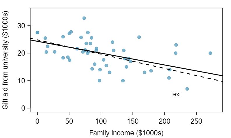
Is the correlation positive or negative in Figure 8.2.2? 2 Larger family incomes are associated with lower amounts of aid, so the correlation will be negative. Using a computer, the correlation can be computed: -0.499.
Subsection 8.2.1 An objective measure for finding the best line
We begin by thinking about what we mean by “best”. Mathematically, we want a line that has small residuals. Perhaps our criterion could minimize the sum of the residual magnitudes:
\begin{gather}
|y_1 - \hat{y}_1| + |y_2-\hat{y}_2| + \dots + |y_n-\hat{y}_n|\label{sumOfAbsoluteValueOfResiduals}\tag{8.2.1}
\end{gather}
which we could accomplish with a computer program. The resulting dashed line shown in Figure 8.2.2 demonstrates this fit can be quite reasonable. However, a more common practice is to choose the line that minimizes the sum of the squared residuals:
\begin{gather}
(y_1 - \hat{y}_1)^2 + (y_2-\hat{y}_2)^2+ \dots + (y_n-\hat{y}_n)^2\label{sumOfSquaresForResiduals}\tag{8.2.2}
\end{gather}
The line that minimizes this least squares criterion is represented as the solid line in Figure 8.2.2. This is commonly called the least squares line. The following are three possible reasons to choose Criterion (8.2.2) over Criterion (8.2.1):
It is the most commonly used method.
Computing the line based on Criterion (8.2.2) is much easier by hand and in most statistical software.
In many applications, a residual twice as large as another residual is more than twice as bad. For example, being off by 4 is usually more than twice as bad as being off by 2. Squaring the residuals accounts for this discrepancy.
The first two reasons are largely for tradition and convenience; the last reason explains why Criterion (8.2.2) is typically most helpful. 3 There are applications where Criterion (8.2.1) may be more useful, and there are plenty of other criteria we might consider. However, this book only applies the least squares criterion.
Subsection 8.2.2 Conditions for the least squares line
When fitting a least squares line, we generally require
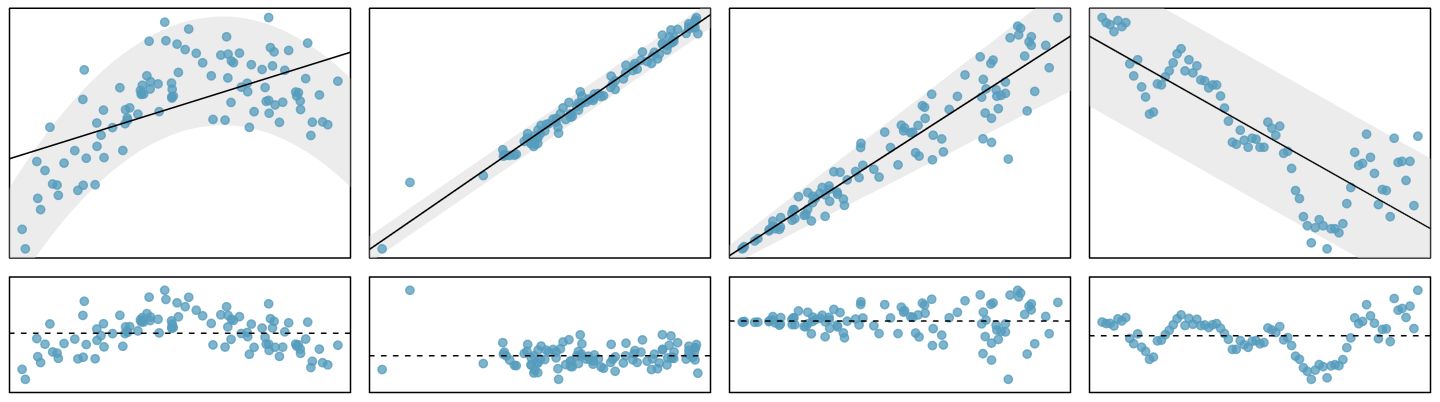
The data should show a linear trend. If there is a nonlinear trend (e.g. left panel of Figure 8.2.4), an advanced regression method from another book or later course should be applied.
Generally the residuals must be nearly normal. When this condition is found to be unreasonable, it is usually because of outliers or concerns about influential points, which we will discuss in greater depth in Section 8.3. An example of non-normal residuals is shown in the second panel of Figure 8.2.4.
The variability of points around the least squares line reidxs roughly constant. An example of non-constant variability is shown in the third panel of Figure 8.2.4.
These conditions are best checked using a residual plot. If a residual plot has no pattern, such as a U-shape or the presence of outliers or non-constant variability in the residuals, then the conditions above may be considered to be satisfied.
TIP: Use a residual plot to determine if a linear model is appropriate
When a residual plot appears as a random cloud of points, a linear model is generally appropriate. If a residual plot has any type of pattern, a linear model is not appropriate.
Be cautious about applying regression to data collected sequentially in what is called a time series. Such data may have an underlying structure that should be considered in a model and analysis.
Guided Practice 8.2.5
Should we have concerns about applying least squares regression to the Elmhurst data in Figure 8.2.2? 4 The trend appears to be linear, the data fall around the line with no obvious outliers, the variance is roughly constant. These are also not time series observations. Least squares regression can be applied to these data.
Subsection 8.2.3 Finding the least squares line
¶For the Elmhurst data, we could write the equation of the least squares regression line as
\begin{gather*}
\widehat{aid} = \beta_0 + \beta_{1}\times family\_income
\end{gather*}
Here the equation is set up to predict gift aid based on a student's family income, which would be useful to students considering Elmhurst. These two values, \(\beta_0\) and \(\beta_1\text{,}\) are the parameters of the regression line.
As in Chapters 4-6, the parameters are estimated using observed data. In practice, this estimation is done using a computer in the same way that other estimates, like a sample mean, can be estimated using a computer or calculator. However, we can also find the parameter estimates by applying two properties of the least squares line:
-
The slope of the least squares line can be estimated by
\begin{gather} b_1 = r\frac{s_y}{s_x}\label{slopeOfLSRLine}\tag{8.2.3} \end{gather}where \(r\) is the correlation between the two variables, and \(s_x\) and \(s_y\) are the sample standard deviations of the explanatory variable and response , respectively.
-
If \(\bar{x}\) is the mean of the horizontal variable (from the data) and \(\bar{y}\) is the mean of the vertical variable, then the point \((\bar{x}, \bar{y})\) is on the least squares line. Plugging this point in for \(x\) and \(y\) in the least squares equation and solving for \(b_0\) gives
\begin{align} \bar{y} \amp = b_0 + b_1\bar{x} \amp \amp b_0=\bar{y}-b_1\bar{x}\label{interceptOfLSRLine}\tag{8.2.4} \end{align}When solving for the \(y\)-intercept, first find the slope, \(b_1\text{,}\) and plug the slope and the point \((\bar{x}, \bar{y})\) into the least squares equation.
We use \(b_0\) and \(b_1\) to represent the point estimates of the parameters \(\beta_0\) and \(\beta_1\text{.}\)
Guided Practice 8.2.6
Table 8.2.7 shows the sample means for the family income and gift aid as $101,800 and $19,940, respectively. Plot the point \((101.8, 19.94)\) on Figure 8.2.2 to verify it falls on the least squares line (the solid line). 5 If you need help finding this location, draw a straight line up from the x-value of 100 (or thereabout). Then draw a horizontal line at 20 (or thereabout). These lines should intersect on the least squares line.
| family income, in $1000s (“\(x\)”) | gift aid, in $1000s (“\(y\)”) | |
| mean | \(\bar{x} = 101.8\) | \(\bar{y} = 19.94\) |
| sd | \(s_x = 63.2\) | \(s_y = 5.46\) |
| \(r=-0.499\) | ||
Guided Practice 8.2.8
Using the summary statistics in Table 8.2.7, compute the slope and \(y\)-intercept for the regression line of gift aid against family income. Write the equation of the regression line. 6 Apply Equation (8.2.3) and Equation (8.2.4) with the summary statistics from Table 8.2.7 to compute the slope and \(y\)-intercept:
\begin{align*}
b_1 \amp = r\frac{s_y}{s_x} = (-0.499)\frac{5.46}{63.2} = -0.0431\\
b_0 \amp = \bar{y} - b_1\bar{x} = 19.94 - (-0.0431)(101.8) = 24.3\\
\hat{y}\amp =24.3 - 0.0431x
\qquad\text{ or } \qquad
\widehat{aid} = 24.3 - 0.0431 \text{ family_income }
\end{align*}
We mentioned earlier that a computer is usually used to compute the least squares line. A summary table based on computer output is shown in Table 8.2.9 for the Elmhurst data. The first column of numbers provides estimates for \({b}_0\) and \({b}_1\text{,}\) respectively. Compare these to the result from Guided Practice 8.2.8.
| Estimate | Std. Error | t value | Pr(\(\gt\)\(|\)t\(|\)) | |
| (Intercept) | 24.3193 | 1.2915 | 18.83 | 0.0000 |
| family_income | -0.0431 | 0.0108 | -3.98 | 0.0002 |
Example 8.2.10
Examine the second, third, and fourth columns in Table 8.2.9. Can you guess what they represent?
Solution
We'll describe the meaning of the columns using the second row, which corresponds to \(\beta_1\text{.}\) The first column provides the point estimate for \(\beta_1\text{,}\) as we calculated in an earlier example: -0.0431. The second column is a standard error for this point estimate: 0.0108. The third column is a \(T\) test statistic for the null hypothesis that \(\beta_1 = 0\text{:}\) \(T=-3.98\text{.}\) The last column is the p-value for the \(T\) test statistic for the null hypothesis \(\beta_1=0\) and a two-sided alternative hypothesis: 0.0002. We will get into more of these details in Section 8.4.
Example 8.2.11
Suppose a high school senior is considering Elmhurst College. Can she simply use the linear equation that we have estimated to calculate her financial aid from the university?
Solution
She may use it as an estimate, though some qualifiers on this approach are important. First, the data all come from one freshman class, and the way aid is determined by the university may change from year to year. Second, the equation will provide an imperfect estimate. While the linear equation is good at capturing the trend in the data, no individual student's aid will be perfectly predicted.
Subsection 8.2.4 Interpreting regression line parameter estimates
Interpreting parameters in a regression model is often one of the most important steps in the analysis.
Example 8.2.12
The slope and intercept estimates for the Elmhurst data are -0.0431 and 24.3. What do these numbers really mean?
Solution
Interpreting the slope parameter is helpful in almost any application. For each additional $1,000 of family income, we would expect a student to receive a net difference of $1,000 \(\times\) (-0.0431) = -$43.10 in aid on average, i.e. $43.10 less. Note that a higher family income corresponds to less aid because the coefficient of family income is negative in the model. We must be cautious in this interpretation: while there is a real association, we cannot interpret a causal connection between the variables because these data are observational. That is, increasing a student's family income may not cause the student's aid to drop. (It would be reasonable to contact the college and ask if the relationship is causal, i.e. if Elmhurst College's aid decisions are partially based on students' family income.)
The estimated intercept \(b_0=24.3\) (in $1000s) describes the average aid if a student's family had no income. The meaning of the intercept is relevant to this application since the family income for some students at Elmhurst is $0. In other applications, the intercept may have little or no practical value if there are no observations where \(x\) is near zero.
Interpreting parameters in a linear model
The slope, \(b_1\text{,}\) describes the average increase or decrease in the \(y\) variable if the explanatory variable \(x\) is one unit larger.
The y-intercept, \(b_0\text{,}\) describes the average or predicted outcome of \(y\) if \(x=0\text{.}\) The linear model must be valid all the way to \(x=0\) for this to make sense, which in many applications is not the case.
Subsection 8.2.5 Extrapolation is treacherous
When those blizzards hit the East Coast this winter, it proved to my satisfaction that global warming was a fraud. That snow was freezing cold. But in an alarming trend, temperatures this spring have risen. Consider this: On February \(6^{th}\) it was 10 degrees. Today it hit almost 80. At this rate, by August it will be 220 degrees. So clearly folks the climate debate rages on.
Stephen Colbert April 6th, 2010 7 http://www.cc.com/video-clips/l4nkoq/the-colbert-report-science-catfight---joe-bastardi-vs--brenda-ekwurzel
Linear models can be used to approximate the relationship between two variables. However, these models have real limitations. Linear regression is simply a modeling framework. The truth is almost always much more complex than our simple line. For example, we do not know how the data outside of our limited window will behave.
Example 8.2.13
Use the model \(\widehat{aid} = 24.3 - 0.0431\times family\_income\) to estimate the aid of another freshman student whose family had income of $1 million.
Solution
Recall that the units of family income are in $1000s, so we want to calculate the aid for \(family\_income = 1000\text{:}\)
\begin{align*}
\widehat{aid} \amp = 24.3 - 0.0431 \times family\_income\\
\widehat{aid}\amp =24.3 - 0.431(1000) = -18.8
\end{align*}
The model predicts this student will have -$18,800 in aid (!). Elmhurst College cannot (or at least does not) require any students to pay extra on top of tuition to attend.
Applying a model estimate to values outside of the realm of the original data is called extrapolation. Generally, a linear model is only an approximation of the real relationship between two variables. If we extrapolate, we are making an unreliable bet that the approximate linear relationship will be valid in places where it has not been analyzed.
Subsection 8.2.6 Using \(R^2\) to describe the strength of a fit
We evaluated the strength of the linear relationship between two variables earlier using the correlation coefficient, \(r\text{.}\) However, it is more common to explain the strength of a linear fit using \(R^2\text{,}\) called R-squared or the explained variance. If provided with a linear model, we might like to describe how closely the data cluster around the linear fit.
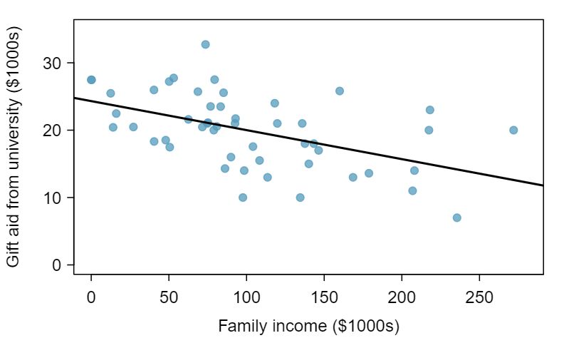
The \(R^2\) of a linear model describes the amount of variation in the response that is explained by the least squares line. For example, consider the Elmhurst data, shown in Figure 8.2.14. The variance of the response variable, aid received, is \(s_{aid}^2=29.8\text{.}\) However, if we apply our least squares line, then this model reduces our uncertainty in predicting aid using a student's family income. The variability in the residuals describes how much variation reidxs after using the model: \(s_{_{RES}}^2 = 22.4\text{.}\) In short, there was a reduction of
\begin{equation*}
\frac{s_{aid}^2 - s_{_{RES}}^2}{s_{aid}^2}
= \frac{29.8 - 22.4}{29.8} = \frac{7.5}{29.8}
= 0.25
\end{equation*}
This is how we compute the \(R^2\) value. 8 \(R^2=1-\frac{s^2_{RES}}{s^2_y}\) It also corresponds to the square of the correlation coefficient, \(r\text{,}\) that is, \(R^2=r^2\text{.}\)
\begin{align*}
R^2 \amp = 0.25 \amp r \amp = -0.499
\end{align*}
\(R^2\) is the explained variance
\(R^2\) is always between 0 and 1, inclusive. It tells us the proportion of variation in the \(y\) values that is explained by a regression model. The higher the value of \(R^2\text{,}\) the better the model “explains” the reponse variable.
Guided Practice 8.2.15
If a linear model has a very strong negative relationship with a correlation of -0.97, how much of the variation in the response is explained by the explanatory variable? 9 About \(R^2 = (-0.97)^2 = 0.94\) or 94% of the variation in aid is explained by the linear model.
Guided Practice 8.2.16
If a linear model has an \(R^2\) or explained variance of 0.94, what is the correlation coefficient? 10 We take the square root of \(R^2\) and get 0.97, but we must be careful, because \(r\) could be 0.97 or -0.97. Without knowing the slope or seeing the scatterplot, we have no way of knowing if \(r\) is positive or negative.
Subsection 8.2.7 Calculator: linear correlation and regression
TI-84: finding \(b_0\text{,}\) \(b_1\text{,}\) \(R^2\text{,}\) and \(r\) for a linear model
MISSINGVIDEOLINK Use STAT, CALC, LinReg(a + bx).
Choose
STAT.Right arrow to
CALC.-
Down arrow and choose
8:LinReg(a+bx).Caution: choosing
4:LinReg(ax+b)will reverse \(a\) and \(b\text{.}\)
Let
XlistbeL1andYlistbeL2(don't forget to enter the \(x\) and \(y\) values in L1 andL2before doing this calculation).Leave
FreqListblank.Leave
Store RegEQblank.Choose Calculate and hit
ENTER, which returns:a\(b_0\text{,}\) the y-intercept of the best fit line b\(b_1\text{,}\) the slope of the best fit line \(r^2\) \(R^2\text{,}\) the explained variance r\(r\text{,}\) the correlation coefficient
TI-83: Do steps 1-3, then enter the \(x\) list and \(y\) list separated by a comma, e.g. LinReg(a+bx) L1, L2, then hit ENTER.
What to do if \(r^2\) and \(r\) do not show up on a TI-83/84
If \(r^2\) and \(r\) do now show up when doing STAT, CALC, LinReg, the diagnostics must be turned on. This only needs to be once and the diagnostics will reidx on.
Hit
2ND0(i.e.CATALOG).Scroll down until the arrow points at
DiagnosticOn.Hit
ENTERandENTERagain. The screen should now say:DiagnosticOnDone
What to do if a TI-83/84 returns: ERR: DIM MISMATCH
This error means that the lists, generally L1 and L2, do not have the same length.
Choose
1:Quit.Choose
STAT,Editand make sure that the lists have the same number of entries.
Casio fx-9750GII: finding \(b_0\text{,}\) \(b_1\text{,}\) \(R^2\text{,}\) and \(r\) for a linear model
Navigate to
STAT(MENUbutton, then hit the2button or selectSTAT).Enter the \(x\) and \(y\) data into 2 separate lists, e.g. \(x\) values in
List 1and \(y\) values inList 2. Observation ordering should be the same in the two lists. For example, if \((5, 4)\) is the second observation, then the second value in the \(x\) list should be 5 and the second value in the \(y\) list should be 4.-
Navigate to
CALC(F2) and thenSET(F6) to set the regression context.To change the
2Var XList, navigate to it, selectList(F1), and enter the proper list number. Similarly, set2Var YListto the proper list.
Hit
EXIT.Select
REG(F3),X(F1), anda+bx(F2), which returns:
If you selecta\(b_0\text{,}\) the y-intercept of the best fit line b\(b_1\text{,}\) the slope of the best fit line r\(r\text{,}\) the correlation coefficient \(r^2\) \(R^2\text{,}\) the explained variance MSeMean squared error, which you can ignore ax+b(F1), theaandbmeanings will be reversed.
fed_spend |
poverty |
|
| 1 | 6.07 | 10.6 |
| 2 | 6.14 | 12.2 |
| 3 | 8.75 | 25.0 |
| 4 | 7.12 | 12.6 |
| 5 | 5.13 | 13.4 |
| 6 | 8.71 | 5.6 |
| 7 | 6.70 | 7.9 |
Guided Practice 8.2.18
Table 8.2.17 contains values of federal spending per capita (rounded to the nearand percent of population in poverty for seven counties. This is a subset of the countyDF data set from Chapter 1. Use a calculator to find the equation of the least squares regression line for this partial data set. 11 \(a=5.136\) and \(b=1.056\text{,}\) therefore \(\hat{y}=5.136 + 1.056x\text{.}\)
Subsection 8.2.8 Categorical predictors with two levels (special topic)
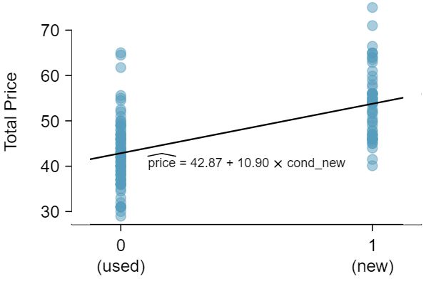
¶Categorical variables are also useful in predicting outcomes. Here we consider a categorical predictor with two levels (recall that a level is the same as a category). We'll consider Ebay auctions for a video game, Mario Kart for the Nintendo Wii, where both the total price of the auction and the condition of the game were recorded. 12 These data were collected in Fall 2009 and may be found at openintro.org/stat. Here we want to predict total price based on game condition, which takes values used and new. A plot of the auction data is shown in Figure 8.2.19.
To incorporate the game condition variable into a regression equation, we must convert the categories into a numerical form. We will do so using an indicator variable called cond_new, which takes value 1 when the game is new and 0 when the game is used. Using this indicator variable, the linear model may be written as
\begin{gather*}
\widehat{price} = \beta_0 + \beta_1 \times \text{cond\_new}
\end{gather*}
The fitted model is summarized in Table 8.2.20, and the model with its parameter estimates is given as
\begin{gather*}
\widehat{price} = 42.87 + 10.90 \times \text{cond\_new}
\end{gather*}
For categorical predictors with just two levels, the linearity assumption will always be satisfied. However, we must evaluate whether the residuals in each group are approximately normal and have approximately equal variance. As can be seen in Figure 8.2.19, both of these conditions are reasonably satisfied by the auction data.
| Estimate | Std. Error | t value | Pr(\(\gt\)\(|\)t\(|\)) | |
| (Intercept) | 42.87 | 0.81 | 52.67 | 0.0000 |
| cond_new | 10.90 | 1.26 | 8.66 | 0.0000 |
Example 8.2.21
Interpret the two parameters estimated in the model for the price of Mario Kart in eBay auctions.
Solution
The intercept is the estimated price when cond_new takes value 0, i.e. when the game is in used condition. That is, the average selling price of a used version of the game is $42.87.
The slope indicates that, on average, new games sell for about $10.90 more than used games.
TIP: Interpreting model estimates for categorical predictors.
The estimated intercept is the value of the response variable for the first category (i.e. the category corresponding to an indicator value of 0). The estimated slope is the average change in the response variable between the two categories.