
Section 3.1 Defining probability
¶Probability Introduction video
A “die”, the singular of dice, is a cube with six faces numbered 1, 2, 3, 4, 5, and 6. What is the chance of getting 1 when rolling a die?
Solution
If the die is fair, then the chance of a 1 is as good as the chance of any other number. Since there are six outcomes, the chance must be 1-in-6 or, equivalently, \(1/6\text{.}\)
Example 3.1.3
What is the chance of getting a 1 or 2 in the next roll?
Solution
1 and 2 constitute two of the six equally likely possible outcomes, so the chance of getting one of these two outcomes must be \(2/6 = 1/3\text{.}\)
Example 3.1.4
What is the chance of getting either 1, 2, 3, 4, 5, or 6 on the next roll?
Solution
100%. The outcome must be one of these numbers.
Example 3.1.5
What is the chance of not rolling a 2?
Solution
Since the chance of rolling a 2 is \(1/6\) or \(16.\bar{6}\%\text{,}\) the chance of not rolling a 2 must be \(100\% - 16.\bar{6}\%=83.\bar{3}\%\) or \(5/6\text{.}\)
Alternatively, we could have noticed that not rolling a 2 is the same as getting a 1, 3, 4, 5, or 6, which makes up five of the six equally likely outcomes and has probability \(5/6\text{.}\)
Example 3.1.6
Consider rolling two dice. If \(1/6^{th}\) of the time the first die is a 1 and \(1/6^{th}\) of those times the second die is a 1, what is the chance of getting two 1s?
Solution
If \(16.\bar{6}\)% of the time the first die is a 1 and \(1/6^{th}\) of those times the second die is also a 1, then the chance that both dice are 1 is \((1/6)\times (1/6)\) or \(1/36\text{.}\)
Subsection 3.1.1 Probability
We use probability to build tools to describe and understand apparent randomness. We often frame probability in terms of a random process giving rise to an outcome.
| Roll a die | \(\rightarrow\) |
1, 2, 3, 4, 5, or 6
|
| Flip a coin | \(\rightarrow\) |
H or T
|
Rolling a die or flipping a coin is a seemingly random process and each gives rise to an outcome.
Probability
The probability of an outcome is the proportion of times the outcome would occur if we observed the random process an infinite number of times.
Probability is defined as a proportion, and it always takes values between 0 and 1 (inclusively). It may also be displayed as a percentage between 0% and 100%.
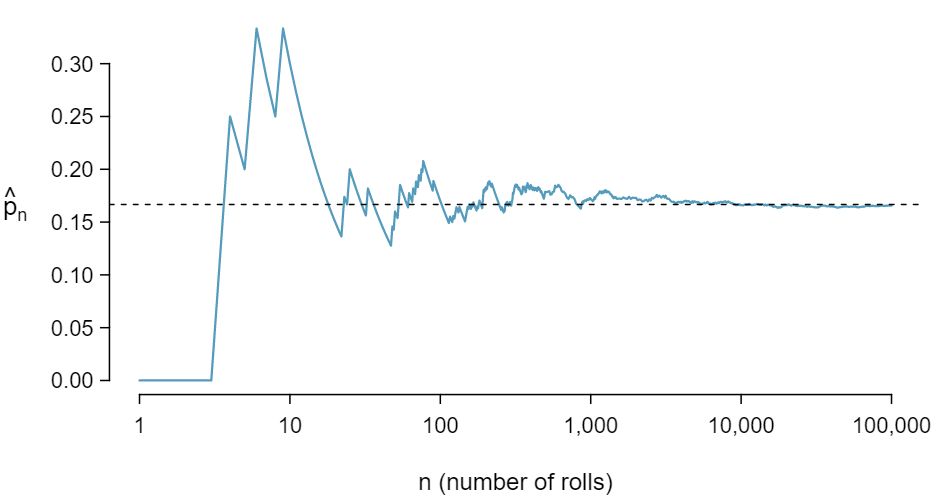
Probability can be illustrated by rolling a die many times. Consider the event “roll a 1”. The relative frequency of an event is the proportion of times the event occurs out of the number of trials. Let \(\hat{p}_n\) be the proportion of outcomes that are 1 after the first \(n\) rolls. As the number of rolls increases, \(\hat{p}_n\) (the relative frequency of rolls) will converge to the probability of rolling a 1, \(p = 1/6\text{.}\) Figure 3.1.7 shows this convergence for 100,000 die rolls. The tendency of \(\hat{p}_n\) to stabilize around \(p\text{,}\) that is, the tendency of the relative frequency to stabilize around the true probability, is described by the Law of Large Numbers.
Law of Large Numbers
As more observations are collected, the observed proportion \(\hat{p}_n\) of occurrences with a particular outcome after \(n\) trials converges to the true probability \(p\) of that outcome.
Occasionally the proportion will veer off from the probability and appear to defy the Law of Large Numbers, as \(\hat{p}_n\) does many times in Figure 3.1.7. However, these deviations become smaller as the number of rolls increases.
Above we write \(p\) as the probability of rolling a 1. We can also write this probability as
\begin{gather*}
P(\text{ rolling a }1)
\end{gather*}
1 \(P(A)\) Probability of outcome \(A\)As we become more comfortable with this notation, we will abbreviate it further. For instance, if it is clear that the process is “rolling a die”, we could abbreviate \(P(\)rolling a 1\()\) as \(P(\)1\()\text{.}\)
Example 3.1.8
Random processes include rolling a die and flipping a coin. (a) Think of another random process. (b) Describe all the possible outcomes of that process. For instance, rolling a die is a random process with potential outcomes 1, 2, ..., 6. 2 Here are four examples. (i) Whether someone gets sick in the next month or not is an apparently random process with outcomes sick and not. (ii) We can generate a random process by randomly picking a person and measuring that person's height. The outcome of this process will be a positive number. (iii) Whether the stock market goes up or down next week is a seemingly random process with possible outcomes up, down, and no_change. Alternatively, we could have used the percent change in the stock market as a numerical outcome. (iv) Whether your roommate cleans her dishes tonight probably seems like a random process with possible outcomes cleans_dishes and leaves_dishes.
What we think of as random processes are not necessarily random, but they may just be too difficult to understand exactly. The fourth example in the footnote solution to Example 3.1.8 suggests a roommate's behavior is a random process. However, even if a roommate's behavior is not truly random, modeling her behavior as a random process can still be useful.
TIP: Modeling a process as random
It can be helpful to model a process as random even if it is not truly random.
Subsection 3.1.2 Disjoint or mutually exclusive outcomes
Two outcomes are called disjoint or mutually exclusive if they cannot both happen in the same trial. For instance, if we roll a die, the outcomes 1 and 2 are disjoint since they cannot both occur on a single roll. On the other hand, the outcomes 1 and “rolling an odd number” are not disjoint since both occur if the outcome of the roll is a 1. The terms disjoint and mutually exclusive are equivalent and interchangeable.
Calculating the probability of disjoint outcomes is easy. When rolling a die, the outcomes 1 and 2 are disjoint, and we compute the probability that one of these outcomes will occur by adding their separate probabilities:
\begin{gather*}
P(1 \text{ or } 2) = P(1) + P(2) = 1/6 + 1/6 = 1/3
\end{gather*}
What about the probability of rolling a 1, 2, 3, 4, 5, or 6? Here again, all of the outcomes are disjoint so we add the probabilities:
\begin{gather*}
P(1\text{ or } 2\text{ or } 3\text{ or } 4 \text{ or } 5 \text{ or } 6)\\
= P(1)+P(2)+P(3)+P(4)+P(5)+P(6)\\
= 1/6 + 1/6 + 1/6 + 1/6 + 1/6 + 1/6 = 1.
\end{gather*}
The Addition Rule guarantees the accuracy of this approach when the outcomes are disjoint.
Addition Rule of disjoint outcomes
If \(A_1\) and \(A_2\) represent two disjoint outcomes, then the probability that one of them occurs is given by
\begin{gather*}
P(A_1\text{ or } A_2) = P(A_1) + P(A_2)
\end{gather*}
If there are many disjoint outcomes \(A_1\text{,}\) ..., \(A_k\text{,}\) then the probability that one of these outcomes will occur is
\begin{gather}
P(A_1) + P(A_2) + \cdots + P(A_k)\label{disjoint_rule}\tag{3.1.1}
\end{gather}
Example 3.1.9
We are interested in the probability of rolling a 1, 4, or 5.
Explain why the outcomes
1,4, and5are disjoint. 3 The random process is a die roll, and at most one of these outcomes can come up. This means they are disjoint outcomes.Apply the Addition Rule for disjoint outcomes to determine \(P(\)
1or4or5\()\text{.}\) 4 \(P(\)1or4or5\()\) =\(P(\)1\()+P(\)4\()+P(\)5\() = \frac{1}{6} + \frac{1}{6} + \frac{1}{6} = \frac{3}{6} = \frac{1}{2}\)
Example 3.1.10
In the email data set in Chapter 2, the number variable described whether no number (labeled none), only one or more small numbers (small), or whether at least one big number appeared in an email (big). Of the 3,921 emails, 549 had no numbers, 2,827 had only one or more small numbers, and 545 had at least one big number.
Are the outcomes
none,small, andbigdisjoint? 5 Yes. Each email is categorized in only one level ofnumber.Determine the proportion of emails with value
smallandbigseparately. 6 Small: \(\frac{2827}{3921} = 0.721\text{.}\) Big: \(\frac{545}{3921} = 0.139\text{.}\)Use the Addition Rule for disjoint outcomes to compute the probability a randomly selected email from the data set has a number in it, small or big. 7 \(P(\)
smallorbig\() = P(\)small\() + P(\)big\() = 0.721 + 0.139 = 0.860\text{.}\)
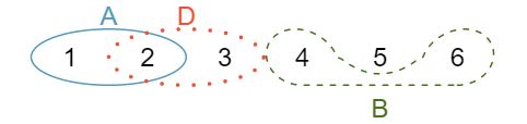
Statisticians rarely work with individual outcomes and instead consider sets or collections of outcomes. Let \(A\) represent the event where a die roll results in 1 or 2 and \(B\) represent the event that the die roll is a 4 or a 6. We write \(A\) as the set of outcomes \(\{\)1, 2\(\}\) and \(B=\{\)4, 6\(\}\text{.}\) These sets are commonly called events. Because \(A\) and \(B\) have no elements in common, they are disjoint events. \(A\) and \(B\) are represented in Figure 3.1.11.
The Addition Rule applies to both disjoint outcomes and disjoint events. The probability that one of the disjoint events \(A\) or \(B\) occurs is the sum of the separate probabilities:
\begin{gather*}
P(A\text{ or } B) = P(A) + P(B) = 1/3 + 1/3 = 2/3
\end{gather*}
Example 3.1.12
Example 3.1.13
Using Figure 3.1.11 as a reference, what outcomes are represented by event \(D\text{?}\) 10 Outcomes
2and3.Are events \(B\) and \(D\) disjoint? 11 Yes, events \(B\) and \(D\) are disjoint because they share no outcomes.
Are events \(A\) and \(D\) disjoint? 12 The events \(A\) and \(D\) share an outcome in common,
2, and so are not disjoint.
Example 3.1.14
In Example 3.1.13, you confirmed \(B\) and \(D\) from Figure 3.1.11 are disjoint. Compute the probability that either event \(B\) or event \(D\) occurs. 13 Since \(B\) and \(D\) are disjoint events, use the Addition Rule: \(P(B\) or \(D) = P(B) + P(D) = \frac{1}{3} + \frac{1}{3} = \frac{2}{3}\text{.}\)
Subsection 3.1.3 Probabilities when events are not disjoint
Let's consider calculations for two events that are not disjoint in the context of a regular deck of 52 cards, represented in Table 3.1.15. If you are unfamiliar with the cards in a regular deck, please see the footnote. 14 The 52 cards are split into four suits: \(\clubsuit\) (club), \(\diamondsuit\) (diamond), \(\heartsuit\) (heart), \(\spadesuit\) (spade). Each suit has its 13 cards labeled: 2, 3, ..., 10, J (jack), Q (queen), K (king), and A (ace). Thus, each card is a unique combination of a suit and a label, e.g. \(\heartsuit\)4 and \(\clubsuit\)J. The 12 cards represented by the jacks, queens, and kings are called face cards. The cards that are \(\diamondsuit\) or \(\heartsuit\) are typically colored red while the other two suits are typically colored black.
| \(\clubsuit 2\) | \(\clubsuit 3\) | \(\clubsuit 4\) | \(\clubsuit 5\) | \(\clubsuit 6\) | \(\clubsuit 7\) | \(\clubsuit 8\) | \(\clubsuit 9\) | \(\clubsuit 10\) | \(\clubsuit\)J | \(\clubsuit\)Q | \(\clubsuit\)K | \(\clubsuit\)A |
| \(\diamondsuit 2\) | \(\diamondsuit 3\) | \(\diamondsuit 4\) | \(\diamondsuit 5\) | \(\diamondsuit 6\) | \(\diamondsuit 7\) | \(\diamondsuit 8\) | \(\diamondsuit 9\) | \(\diamondsuit 10\) | \(\diamondsuit\)J | \(\diamondsuit\)Q | \(\diamondsuit\)K | \(\diamondsuit\)A |
| \(\heartsuit 2\) | \(\heartsuit 3\) | \(\heartsuit 4\) | \(\heartsuit 5\) | \(\heartsuit 6\) | \(\heartsuit 7\) | \(\heartsuit 8\) | \(\heartsuit 9\) | \(\heartsuit 10\) | \(\heartsuit\)J | \(\heartsuit\)Q | \(\heartsuit\)K | \(\heartsuit\)A |
| \(\spadesuit 2\) | \(\spadesuit 3\) | \(\spadesuit 4\) | \(\spadesuit 5\) | \(\spadesuit 6\) | \(\spadesuit 7\) | \(\spadesuit 8\) | \(\spadesuit 9\) | \(\spadesuit 10\) | \(\spadesuit\)J | \(\spadesuit\)Q | \(\spadesuit\)K | \(\spadesuit\)A |
Guided Practice 3.1.16
What is the probability that a randomly selected card is a diamond? 15 There are 52 cards and 13 diamonds. If the cards are thoroughly shuffled, each card has an equal chance of being drawn, so the probability that a randomly selected card is a diamond is \(P({\color{redcards}\diamondsuit}) = \frac{13}{52} = 0.250\text{.}\)
What is the probability that a randomly selected card is a face card? 16 Likewise, there are 12 face cards, so \(P(\)face card\() = \frac{12}{52} = \frac{3}{13} = 0.231\text{.}\)
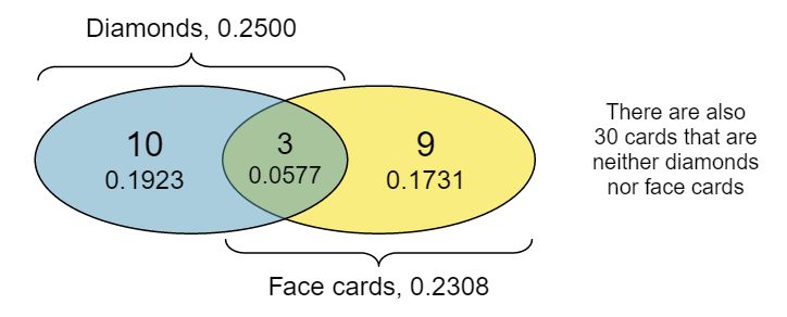
Venn diagrams are useful when outcomes can be categorized as “in” or “out” for two or three variables, attributes, or random processes. The Venn diagram in Figure 3.1.17 uses a circle to represent diamonds and another to represent face cards. If a card is both a diamond and a face card, it falls into the intersection of the circles. If it is a diamond but not a face card, it will be in part of the left circle that is not in the right circle (and so on). The total number of cards that are diamonds is given by the total number of cards in the diamonds circle: \(10+3=13\text{.}\) The probabilities are also shown (e.g. \(10/52 = 0.1923\)).
Example 3.1.18
Using the Venn diagram, verify \(P(\)face card\() = 12/52=3/13\text{.}\) 17 The Venn diagram shows face cards split up into “face card but not \(\diamondsuit\)” and “face card and \(\diamondsuit\)”. Since these correspond to disjoint events, \(P(\)face card\()\) is found by adding the two corresponding probabilities: \(\frac{3}{52} + \frac{9}{52} = \frac{12}{52} = \frac{3}{13}\text{.}\)
Let \(A\) represent the event that a randomly selected card is a diamond and \(B\) represent the event that it is a face card. How do we compute \(P(A\) or \(B)\text{?}\) Events \(A\) and \(B\) are not disjoint — the cards \(J\diamondsuit\text{,}\) \(Q\diamondsuit\text{,}\) and \(K\diamondsuit\) fall into both categories — so we cannot use the Addition Rule for disjoint events. Instead we use the Venn diagram. We start by adding the probabilities of the two events:
\begin{gather*}
P(A) + P(B) = P({\color{redcards}\diamondsuit}) + P(\text{ face card } ) = 13/52 + 12/52
\end{gather*}
However, the three cards that are in both events were counted twice, once in each probability. We must correct this double counting:
\begin{align*}
P(A\text{ or } B) \amp = P({\color{redcards}\diamondsuit}) + P(\text{ face card } )\\
\amp = P({\color{redcards}\diamondsuit}) + P(\text{ face card } ) - P({\color{redcards}\diamondsuit} \text{ and face card } )\\
\amp = 13/52 + 12/52 - 3/52\\
\amp = 22/52 = 11/26
\end{align*}
() is an example of the General Addition Rule.
General Addition Rule
If \(A\) and \(B\) are any two events, disjoint or not, then the probability that A or B will occur is
\begin{gather}
P(A\text{ or } B) = P(A) + P(B) - P(A\text{ and } B)\label{gen_add_rule}\tag{3.1.2}
\end{gather}
where \(P(A\) and \(B)\) is the probability that both events occur.
TIP: Symbolic notation for “and” and “or”
The symbol \(\cap\) means intersection and is equivalent to “and”.
The symbol \(\cup\) means union and is equivalent to “or”.
It is common to see the General Addition Rule written as
\begin{gather}
P(A \cup B) = P(A) + P(B) - P(A \cap B)\label{gen_add_rule_ver_two}\tag{3.1.3}
\end{gather}
TIP: “or” is inclusive
When we write, “or” in statistics, we mean “and/or” unless we explicitly state otherwise. Thus, \(A\) or \(B\) occurs means \(A\text{,}\) \(B\text{,}\) or both \(A\) and \(B\) occur. This is equivalent to at least one of \(A\) or \(B\) occurring.
Example 3.1.19
If \(A\) and \(B\) are disjoint, describe why this implies \(P(A\) and \(B) = 0\text{.}\) 18 If \(A\) and \(B\) are disjoint, \(A\) and \(B\) can never occur simultaneously.
Using part (1), verify that the General Addition Rule simplifies to the simpler Addition Rule for disjoint events if \(A\) and \(B\) are disjoint. 19 If \(A\) and \(B\) are disjoint, then the last term of Equation (3.1.2) is 0 (see part (a)) and we are left with the Addition Rule for disjoint events.
Example 3.1.20
In the email data set with 3,921 emails, 367 were spam, 2,827 contained some small numbers but no big numbers, and 168 had both characteristics. Create a Venn diagram for this setup. 20 Both the counts and corresponding probabilities (e.g. \(2659/3921 = 0.678\)) are shown. Notice that the number of emails represented in the left circle corresponds to \(2659 + 168 = 2827\text{,}\) and the number represented in the right circle is \(168 + 199 = 367\text{.}\) 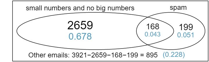
Example 3.1.21
Use your Venn diagram from Example 3.1.20 to determine the probability a randomly drawn email from the
emaildata set is spam and had small numbers (but not big numbers). 21 The solution is represented by the intersection of the two circles: 0.043.What is the probability that the email had either of these attributes? 22 This is the sum of the three disjoint probabilities shown in the circles: \(0.678 + 0.043 + 0.051 = 0.772\text{.}\)
Subsection 3.1.4 Complement of an event
Rolling a die produces a value in the set \(\{\)1, 2, 3, 4, 5, 6\(\}\text{.}\) This set of all possible outcomes is called the sample space (\(S\)) 23 \(S\) Sample space for rolling a die. We often use the sample space to examine the scenario where an event does not occur.
Let \(D=\{\)2, 3\(\}\) represent the event that the outcome of a die roll is 2 or 3. Then the complement 24 \(A^c\) Complement of outcome \(A\) of \(D\) represents all outcomes in our sample space that are not in \(D\text{,}\) which is denoted by \(D^c = \{\)1, 4, 5, 6\(\}\text{.}\) That is, \(D^c\) is the set of all possible outcomes not already included in \(D\text{.}\) Figure 3.1.22 shows the relationship between \(D\text{,}\) \(D^c\text{,}\) and the sample space \(S\text{.}\)
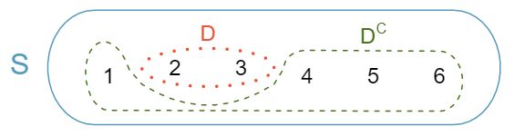
2, 3\(\}\) and its complement, \(D^c = \{\)1, 4, 5, 6\(\}\text{.}\) \(S\) represents the sample space, which is the set of all possible events.Guided Practice 3.1.23
Compute \(P(D^c) = P(\)rolling a
1,4,5, or6\()\text{.}\) 25 The outcomes are disjoint and each has probability \(1/6\text{,}\) so the total probability is \(4/6=2/3\text{.}\)What is \(P(D) + P(D^c)\text{?}\) 26 We can also see that \(P(D)=\frac{1}{6} + \frac{1}{6} = 1/3\text{.}\) Since \(D\) and \(D^c\) are disjoint, \(P(D) + P(D^c) = 1\text{.}\)
Guided Practice 3.1.24
Events \(A=\{\)1, 2\(\}\) and \(B=\{\)4, 6\(\}\) are shown in Figure 3.1.11 on Figure 3.1.11.
Write out what \(A^c\) and \(B^c\) represent. 27 \(A^c=\{\)
3,4,5,6\(\}\) and \(B^c=\{\)1,2,3,5\(\}\text{.}\)Compute \(P(A^c)\) and \(P(B^c)\text{.}\) 28 Noting that each outcome is disjoint, add the individual outcome probabilities to get \(P(A^c)=2/3\) and \(P(B^c)=2/3\text{.}\)
Compute \(P(A)+P(A^c)\) and \(P(B)+P(B^c)\) 29 \(A\) and \(A^c\) are disjoint, and the same is true of \(B\) and \(B^c\text{.}\) Therefore, \(P(A) + P(A^c) = 1\) and \(P(B) + P(B^c) = 1\text{.}\)
An event \(A\) together with its complement \(A^c\) comprise the entire sample space. Because of this we can say that \(P(A) + P(A^c) = 1\text{.}\)
Complement
The complement of event \(A\) is denoted \(A^c\text{,}\) and \(A^c\) represents all outcomes not in \(A\text{.}\) \(A\) and \(A^c\) are mathematically related:
\begin{gather}
P(A) + P(A^c) = 1, \text{ i.e. } P(A) = 1-P(A^c)\label{complement_rule}\tag{3.1.4}
\end{gather}
In simple examples, computing \(A\) or \(A^c\) is feasible in a few steps. However, using the complement can save a lot of time as problems grow in complexity.
Example 3.1.25
A die is rolled 10 times.
What is the complement of getting at least one 6 in 10 rolls of the die? 30 The complement of getting at least one 6 in ten rolls of a die is getting zero 6's in the 10 rolls.
What is the complement of getting at most three 6's in 10 rolls of the die? 31 The complement of getting at most three 6's in 10 rolls is getting four, five, ..., nine, or ten 6's in 10 rolls.
Subsection 3.1.5 Independence
¶Just as variables and observations can be independent, random processes can be independent, too. Two processes are independent if knowing the outcome of one provides no useful information about the outcome of the other. For instance, flipping a coin and rolling a die are two independent processes — knowing the coin was heads does not help determine the outcome of a die roll. On the other hand, stock prices usually move up or down together, so they are not independent.
Example 3.1.6 provides a basic example of two independent processes: rolling two dice. We want to determine the probability that both will be 1. Suppose one of the dice is red and the other white. If the outcome of the red die is a 1, it provides no information about the outcome of the white die. We first encountered this same question in Example 3.1.6, where we calculated the probability using the following reasoning: \(1/6^{th}\) of the time the red die is a 1, and \(1/6^{th}\) of those times the white die will also be 1. This is illustrated in Figure 3.1.26. Because the rolls are independent, the probabilities of the corresponding outcomes can be multiplied to get the final answer: \((1/6)\times(1/6)=1/36\text{.}\) This can be generalized to many independent processes.
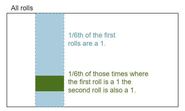
1. Then \(1/6^{th}\) of those times, the second roll will also be a 1.Example 3.1.27
What if there was also a blue die independent of the other two? What is the probability of rolling the three dice and getting all 1s?
Solution
The same logic applies from Example 3.1.6. If \(1/36^{th}\) of the time the white and red dice are both 1, then \(1/6^{th}\) of those times the blue die will also be 1, so multiply: {
\begin{gather*}
P(\text{ white}=1 \text{ and red }=1 \text{ and blue}=1)\\
= P(\text{ white }=1)\times P(\text{ red }=1) \times P(\text{blue }=1)\\
= (1/6)\times (1/6)\times (1/6)
= 1/216
\end{gather*}
Example 3.1.6 and Example 3.1.27 illustrate what is called the Multiplication Rule for independent processes.
Multiplication Rule for independent processes
If \(A\) and \(B\) represent events from two different and independent processes, then the probability that both \(A\) and \(B\) occur can be calculated as the product of their separate probabilities:
\begin{gather}
P(A \text{ and } B) = P(A) \times P(B)\label{eqForIndependentEvents}\tag{3.1.5}
\end{gather}
Similarly, if there are \(k\) events \(A_1\text{,}\) ..., \(A_k\) from \(k\) independent processes, then the probability they all occur is
\begin{gather*}
P(A_1) \times P(A_2)\times \cdots \times P(A_k)
\end{gather*}
Guided Practice 3.1.28
About 9% of people are left-handed. Suppose 2 people are selected at random from the U.S. population. Because the sample size of 2 is very small relative to the population, it is reasonable to assume these two people are independent.
What is the probability that both are left-handed? 32 The probability the first person is left-handed is \(0.09\text{,}\) which is the same for the second person. We apply the Multiplication Rule for independent processes to determine the probability that both will be left-handed: \(0.09\times 0.09 = 0.0081\text{.}\)
What is the probability that both are right-handed? 33 It is reasonable to assume the proportion of people who are ambidextrous (both right and left handed) is nearly 0, which results in \(P(\)right-handed\()=1-0.09=0.91\text{.}\) Using the same reasoning as in part (a), the probability that both will be right-handed is \(0.91\times 0.91 = 0.8281\text{.}\)
Guided Practice 3.1.29
Suppose 5 people are selected at random. 34 The abbreviations RH and LH are used for right-handed and left-handed, respectively. Since each are independent, we apply the Multiplication Rule for independent processes:
What is the probability that all are right-handed? 35
\begin{gather*} P(\text{ all five are RH })\\ = P(\text{ first } = \text{ RH }, \text{ second } = \text{ RH}, ..., \text{ fifth } = \text{ RH })\\ = P(\text{ first } = \text{ RH}) \times P(\text{ second } = \text{ RH } \times ... \times P(\text{ fifth } = \text{ RH })\\ = 0.91\times 0.91\times 0.91\times 0.91\times 0.91 = 0.624 \end{gather*}What is the probability that all are left-handed? 36 Using the same reasoning as in (a), \(0.09\times 0.09\times 0.09\times 0.09\times 0.09 = 0.0000059\)
What is the probability that not all of the people are right-handed? 37 Use the complement, \(P(\)all five are
RH\()\text{,}\) to answer this question:\begin{gather*} P(\text{ not all RH}) = 1 - P(\text{all RH}) = 1 - 0.624 = 0.376 \end{gather*}
Suppose the variables handedness and gender are independent, i.e. knowing someone's gender provides no useful information about their handedness and vice-versa. Then we can compute whether a randomly selected person is right-handed and female 38 The actual proportion of the U.S. population that is female is about 50%, and so we use 0.5 for the probability of sampling a woman. However, this probability does differ in other countries. using the Multiplication Rule:
\begin{align*}
P(\text{ right-handed and female } ) \amp =P(\text{ right-handed } ) \times P(\text{ female } )\\
\amp = 0.91 \times 0.50 = 0.455
\end{align*}
Guided Practice 3.1.30
Three people are selected at random.
What is the probability that the first person is male and right-handed? 39 This can be written in probability notation as \(P(\)a randomly selected person is male and right-handed\()=0.455\)
What is the probability that the first two people are male and right-handed? 40 0.207.
What is the probability that the third person is female and left-handed? 41 0.045.
What is the probability that the first two people are male and right-handed and the third person is female and left-handed? 42 0.0093.
Sometimes we wonder if one outcome provides useful information about another outcome. The question we are asking is, are the occurrences of the two events independent? We say that two events \(A\) and \(B\) are independent if they satisfy Equation (3.1.5).
Example 3.1.31
If we shuffle up a deck of cards and draw one, is the event that the card is a heart independent of the event that the card is an ace?
Solution
The probability the card is a heart is \(1/4\) and the probability that it is an ace is \(1/13\text{.}\) The probability the card is the ace of hearts is \(1/52\text{.}\) We check whether Equation (3.1.5) is satisfied:
\begin{gather*}
P(\heartsuit)\times P(\text{ ace } ) = \frac{1}{4}\times \frac{1}{13} = \frac{1}{52}
= P(\heartsuit\text{ and ace } )
\end{gather*}
Because the equation holds, the event that the card is a heart and the event that the card is an ace are independent events.