Subsection4.2.1The mean and standard deviation of \(\bar{x}\)
In this section we consider a data set called run10, which represents all 16,924 runners who finished the 2012 Cherry Blossom 10 mile run in Washington, DC. 1 MISSINGoiRedirect Part of this data set is shown in Table 4.2.2, and the variables are described in Table 4.2.3.
ID
time
age
gender
state
1
92.25
38.00
M
MD
2
106.35
33.00
M
DC
3
89.33
55.00
F
VA
4
113.50
24.00
F
VA
\(\vdots\)
\(\vdots\)
\(\vdots\)
\(\vdots\)
\(\vdots\)
16923
122.87
37.00
F
VA
16924
93.30
27.00
F
DC
Table4.2.2 Six observations from the run10 data set.
variable
description
time
Ten mile run time, in minutes
age
Age, in years
gender
Gender (M for male, F for female)
state
Home state (or country if not from the US)
Table4.2.3 Variables and their descriptions for the run10 data set.
These data are special because they include the results for the entire population of runners who finished the 2012 Cherry Blossom Run. We took a simple random sample of this population, which is represented in Table 4.2.4. A histogram summarizing the time variable in the run10Samp data set is shown in Figure 4.2.5.
ID
time
age
gender
state
1983
88.31
59
M
MD
8192
100.67
32
M
VA
11020
109.52
33
F
VA
\(\vdots\)
\(\vdots\)
\(\vdots\)
\(\vdots\)
\(\vdots\)
1287
89.49
26
M
DC
Table4.2.4 Four observations for the run10Samp data set, which represents a simple random sample of 100 runners from the 2012 Cherry Blossom Run.
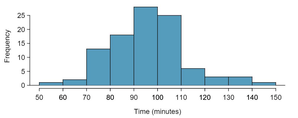
Figure4.2.5 Histogram of time for a single sample of size 100. The average of the sample is in the mid-90s and the standard deviation of the sample \(s\approx 16\) minutes.
From the random sample represented in run10Samp, we guessed the average time it takes to run 10 miles is 95.61 minutes. Suppose we take another random sample of 100 individuals and take its mean: 95.30 minutes. Suppose we took another (93.43 minutes) and another (94.16 minutes), and so on. If we do this many many times — which we can do only because we have the entire population data set — we can build up a sampling distribution for the sample mean when the sample size is 100, shown in Figure 4.2.6.
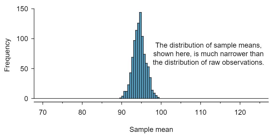
Figure4.2.6 A histogram of 1000 sample means for run time, where the samples are of size \(n=100\text{.}\) This histogram approximates the true sampling distribution of the sample mean, with mean \(\mu_{\bar{x}}\) and standard deviation \(\sigma_{\bar{x}}\text{.}\)
Sampling distribution
The sampling distribution represents the distribution of the point estimates based on samples of a fixed size from a certain population. It is useful to think of a point estimate as being drawn from such a distribution. Understanding the concept of a sampling distribution is central to understanding statistical inference.
The sampling distribution shown in Figure 4.2.6 is unimodal and approximately symmetric. It is also centered exactly at the true population mean: \(\mu=94.52\text{.}\) Intuitively, this makes sense. The sample mean should be an unbiased estimator of the population mean. Because we are considering the distribution of the sample mean, we will use \(\mu_{\bar{x}} = 94.52\) to describe the true mean of this distribution.
We can see that the sample mean has some variability around the population mean, which can be quantified using the standard deviation of this distribution of sample means. The standard deviation of the sample mean tells us how far the typical estimate is away from the actual population mean, 94.52 minutes. It also describes the typical error of a single estimate, and is denoted by the symbol \(\sigma_{\bar{x}}\text{.}\)
Standard deviation of an estimate
The standard deviation associated with an estimate describes the typical error or uncertainty associated with the estimate.
Looking at Figure 4.2.5 and Figure 4.2.6, we see that the standard deviation of the sample mean with \(n=100\) is much smaller than the standard deviation of a single sample. Interpret this statement and explain why it is true.
The variation from one sample mean to another sample mean is much smaller than the variation from one individual to another individual. This makes sense because when we average over 100 values, the large and small values tend to cancel each other out. While many individuals have a time under 90 minutes, it would be unlikely for the average of 100 runners to be less than 90 minutes.
Would you rather use a small sample or a large sample when estimating a parameter? Why? 2 Consider two random samples: one of size 10 and one of size 1000. Individual observations in the small sample are highly influential on the estimate while in larger samples these individual observations would more often average each other out. The larger sample would tend to provide a more accurate estimate.
Using your reasoning from (a), would you expect a point estimate based on a small sample to have smaller or larger standard deviation than a point estimate based on a larger sample? 3 If we think an estimate is better, we probably mean it typically has less error. Based on (a), our intuition suggests that a larger sample size corresponds to a smaller standard deviation.
When considering how to calculate the standard deviation of a sample mean, there is one problem: there is no obvious way to estimate this from a single sample. However, statistical theory provides a helpful tool to address this issue.
In the sample of 100 runners, the standard deviation of the sample mean is equal to one-tenth of the population standard deviation: \(15.93/10 = 1.59\text{.}\) In other words, the standard deviation of the sample mean based on 100 observations is equal to
where \(\sigma_{x}\) is the standard deviation of the individual observations. This is no coincidence. We can show mathematically that this equation is correct when the observations are independent using the probability tools of Section 3.5.
Computing SD for the sample mean
Given \(n\) independent observations from a population with standard deviation \(\sigma\text{,}\) the standard deviation of the sample mean is equal to
The average of the runners' ages is 35.05 years with a standard deviation of \(\sigma = 8.97\text{.}\) A simple random sample of 100 runners is taken.
What is the standard deviation of the sample mean? 4 Use Equation (4.2.1) with the population standard deviation to compute the standard deviation of the sample mean: \(SD_{\bar{y}} = 8.97/\sqrt{100} = 0.90\) years
Would you be surprised to get a sample of size 100 with an average of 36 years? 5 It would not be surprising. 36 years is about 1 standard deviation from the true mean of 35.05. Based on the 68, 95 rule, we would get a sample mean at least this far away from the true mean approximately \(100\% - 68\% = 32\%\) of the time.
Would you be more trusting of a sample that has 100 observations or 400 observations? 6 Extra observations are usually helpful in understanding the population, so a point estimate with 400 observations seems more trustworthy.
We want to show mathematically that our estimate tends to be better when the sample size is larger. If the standard deviation of the individual observations is 10, what is our estimate of the standard deviation of the mean when the sample size is 100? What about when it is 400? 7 The standard deviation of the mean when the sample size is 100 is given by \(SD_{100} = 10/\sqrt{100} = 1\text{.}\) For 400: \(SD_{400} = 10/\sqrt{400} = 0.5\text{.}\) The larger sample has a smaller standard deviation of the mean.
Explain how your answer to (b) mathematically justifies your intuition in part (a). 8 The standard deviation of the mean of the sample with 400 observations is lower than that of the sample with 100 observations. The standard deviation of \(\bar{x}\) describes the typical error, and since it is lower for the larger sample, this mathematically shows the estimate from the larger sample tends to be better — though it does not guarantee that every large sample will provide a better estimate than a particular small sample.
Subsection4.2.2Examining the Central Limit Theorem
In Figure 4.2.6, the sampling distribution of the sample mean looks approximately normally distributed. Will the sampling distribution of a mean always be nearly normal? To address this question, we will investigate three cases to see roughly when the approximation is reasonable.
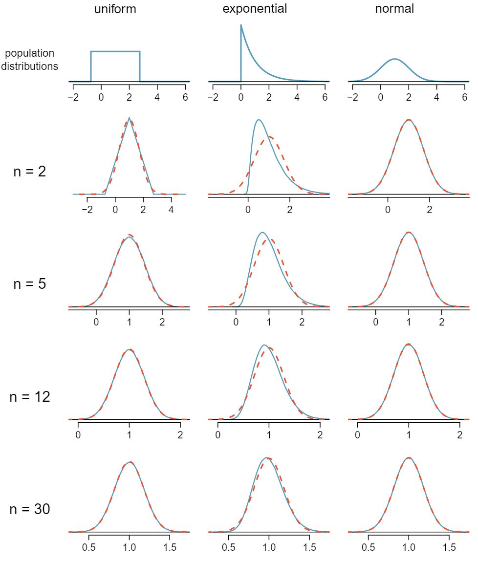
We consider three data sets: one from a uniform distribution, one from an exponential distribution, and the other from a normal distribution. These distributions are shown in the top panels of Figure 4.2.11. The uniform distribution is symmetric, and the exponential distribution may be considered as having moderate skew since its right tail is relatively short (few outliers).
Figure4.2.11 Sampling distributions for the mean at different sample sizes and for three different distributions. The dashed red lines show normal distributions.
The left panel in the \(n=2\) row represents the sampling distribution of \(\bar{x}\) if it is the sample mean of two observations from the uniform distribution shown. The dashed line represents the closest approximation of the normal distribution. Similarly, the center and right panels of the \(n=2\) row represent the respective distributions of \(\bar{x}\) for data from exponential and log-normal distributions.
Examine the distributions in each row of Figure 4.2.11. What do you notice about the sampling distribution of the mean as the sample size, \(n\text{,}\) becomes larger? 9 The normal approximation becomes better as larger samples are used. However, in the case when the population is normally distributed, the normal distribution of the sample mean is normal for all sample sizes.
Yes, the sampling distributions when \(n = 30\) all look very much like the normal distribution.
However, the more non-normal a population distribution, the larger a sample size is necessary for the sampling distribution to look nearly normal.
Determining if the sample mean is normally distributed
If the population is normal, the sampling distribution of \(\bar{x}\) will be normal for any sample size.
The less normal the population, the larger \(n\) needs to be for the sampling distribution of \(\bar{x}\) to be nearly normal. However, a good rule of thumb is that for almost all populations, the sampling distribution of \(\bar{x}\) will be approximately normal if \(n \ge 30\text{.}\)
This brings us to the Central Limit Theorem, the most fundamental theorem in Statistics.
Central Limit Theorem
When taking a random sample of independent observations from a population with a fixed mean and standard deviation, the distribution of \(\bar{x}\) approaches the normal distribution as \(n\) increases.
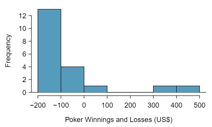
Sometimes we do not know what the population distribution looks like. We have to infer it based on the distribution of a single sample. Figure 4.2.15 shows a histogram of 20 observations. These represent winnings and losses from 20 consecutive days of a professional poker player. Based on this sample data, can the normal approximation be applied to the distribution of the sample mean?
We should consider each of the required conditions.
These are referred to as time series data, because the data arrived in a particular sequence. If the player wins on one day, it may influence how she plays the next. To make the assumption of independence we should perform careful checks on such data.
The sample size is 20, which is smaller than 30.
There are two outliers in the data, both quite extreme, which suggests the population may not be normal and instead may be very strongly skewed or have distant outliers. Outliers can play an important role and affect the distribution of the sample mean and the estimate of the standard deviation of the sample mean.
Since we should be skeptical of the independence of observations and the extreme upper outliers pose a challenge, we should not use the normal model for the sample mean of these 20 observations. If we can obtain a much larger sample, then the concerns about skew and outliers would no longer apply.
Figure4.2.15 Sample distribution of poker winnings. These data include two very clear outliers. These are problematic when considering the normality of the sample mean. For example, outliers are often an indicator of very strong skew.
Caution: Examine data structure when considering independence
Some data sets are collected in such a way that they have a natural underlying structure between observations, e.g. when observations occur consecutively. Be especially cautious about independence assumptions regarding such data sets.
Caution: Watch out for strong skew and outliers
Strong skew in the population is often identified by the presence of clear outliers in the data. If a data set has prominent outliers, then a larger sample size will be needed for the sampling distribution of \(\bar{x}\) to be normal. There are no simple guidelines for what sample size is big enough for each situation. However, we can use the rule of thumb that, in general, an \(n\) of at least 30 is sufficient for most cases.
Subsection4.2.3Normal approximation for the sampling distribution of \(\bar{x}\)
At the beginning of this chapter, we used normal approximation for populations or for data that had an approximately normal distribution. When appropriate conditions are met, we can also use the normal approximation to estimate probabilities about a sample average. We must remember to verify that the conditions are met and use the mean \(\mu_{\bar{x}}\) and standard deviation \(\sigma_{\bar{x}}\) for the sampling distribution of the sample average.
TIP: Three important facts about the distribution of a sample mean \(\bar{x}\)
Consider taking a simple random sample from a large population.
The mean of a sample mean is denoted by \(\mu_{\bar{x}}\text{,}\) and it is equal to \(\mu\text{.}\)
The SD of a sample mean is denoted by \(\sigma_{\bar{x}}\text{,}\) and it is equal to \(\frac{\sigma}{\sqrt{n}}\text{.}\)
When the population is normal or when \(n\ge 30\text{,}\) the sample mean closely follows a normal distribution.
In the 2012 Cherry Blossom 10 mile run, the average time for all of the runners is 94.52 minutes with a standard deviation of 8.97 minutes. The distribution of run times is approximately normal. Find the probabiliy that a randomly selected runner completes the run in less than 90 minutes.
Here, \(n=20\lt 30\text{,}\) but the distribution of the population, that is, the distribution of run times is stated to be approximately normal. Because of this, the sampling distribution will be normal for any sample size.
The average of all the runners' ages is 35.05 years with a standard deviation of \(\sigma = 8.97\text{.}\) The distribution of age is somewhat skewed. What is the probability that a randomly selected runner is older than 37 years?
Because the distribution of age is skewed and is not normal, we cannot use normal approximation for this problem. In order to answer this question, we would need to look at all of the data.
What is the probability that the average of 50 randomly selected runners is greater than 37 years? 10 Because \(n=50\ge 30\text{,}\) the sampling distribution of the mean is approximately normal, so we can use normal approximation for this problem. The mean is given as 35.05 years.
There is a 6.2% chance that the average age of 50 runners will be greater than 37.
TIP: Remember to divide by \(\sqrt{n}\)
When finding the probability that an average or mean is greater or less than a particular value, remember to divide the standard deviation of the population by \(\sqrt{n}\) to calculate the correct SD.