
Section 5.3 Introducing hypothesis testing
OpenIntro: Hypothesis Testing
Suppose your professor splits the students in class into two groups: students on the left and students on the right. If \(\hat{p}_{_L}\) and \(\hat{p}_{_R}\) represent the proportion of students who own an Apple product on the left and right, respectively, would you be surprised if \(\hat{p}_{_L}\) did not exactly equal \(\hat{p}_{_R}\text{?}\)
Solution
While the proportions would probably be close to each other, they are probably not exactly the same. We would probably observe a small difference due to chance.
Studying randomness of this form is a key focus of statistics. How large would the observed difference in these two proportions need to be for us to believe that there is a real difference in Apple ownership? In this section, we'll explore this type of randomness in the context of an unknown proportion, and we'll learn new tools and ideas that will be applied throughout the rest of the book.
Subsection 5.3.1 Case study: medical consultant
People providing an organ for donation sometimes seek the help of a special medical consultant. These consultants assist the patient in all aspects of the surgery, with the goal of reducing the possibility of complications during the medical procedure and recovery. Patients might choose a consultant based in part on the historical complication rate of the consultant's clients.
One consultant tried to attract patients by noting the overall complication rate for liver donor surgeries in the US is about 10%, but her clients have had only 9 complications in the 142 liver donor surgeries she has facilitated. She claims this is strong evidence that her work meaningfully contributes to reducing complications (and therefore she should be hired!).
Example 5.3.3
We will let \(p\) represent the true complication rate for liver donors working with this consultant. Estimate \(p\) using the data, and label this value \(\hat{p}\text{.}\)
Solution
The sample proportion for the complication rate is 9 complications divided by the 142 surgeries the consultant has worked on: \(\hat{p} = 9 / 142 = 0.063\text{.}\)
Example 5.3.4
Is it possible to prove that the consultant's work reduces complications?
Solution
No. The claim implies that there is a causal connection, but the data are observational. For example, maybe patients who can afford a medical consultant can afford better medical care, which can also lead to a lower complication rate.
Example 5.3.5
While it is not possible to assess the causal claim, it is still possible to ask whether the low complication rate of \(\hat{p} = 0.063\) provides evidence that the consultant's true complication rate is different than the US complication rate. Why might we be tempted to immediately conclude that the consultant's true complication rate is different than the US complication rate? Can we draw this conclusion?
Solution
Her sample complication rate is \(\hat{p} = 0.063\text{,}\) which is 0.037 lower than the US complication rate of 10%. However, we cannot yet be sure if the observed difference represents a real difference or is just the result of random variation. We wouldn't expect the sample proportion to be exactly 0.10, even if the truth was that her real complication rate was 0.10.
Subsection 5.3.2 Setting up the null and alternate hypothesis
We can set up two competing hypotheses about the consultant's true complication rate. The first is call the null hypothesis and represents either a skeptical perspective or a perspective of no difference. The second is called the alternative hypothesis (or alternate hypothesis) and represents a new perspective such as the possibility that there has been a change or that there is a treatment effect in an experiment.
Null and alternative hypotheses
The null hypothesis is abbreviated \(H_0\text{.}\) It states that nothing has changed and that any deviation from what was expected is due to chance error.
The alternative hypothesis is abbreviated \(H_A\text{.}\) It asserts that there has been a change and that the observed deviation is too large to be explained by chance alone.
Example 5.3.6
Identify the null and alternative claim regarding the consultant's complication rate.
Solution
\(H_0\text{:}\) The true complication rate for the consultant's clients is the same as the US complication rate of 10%.
\(H_A\text{:}\) The true complication rate for the consultant's clients is different than 10%.
Often it is convenient to write the null and alternative hypothesis in mathematical or numerical terms. To do so, we must first identify the quantity of interest. This quantity of interest is known as the parameter for a hypothesis test.
Parameters and point estimates
A parameter for a hypothesis test is the “true” value of the population of interest. When the parameter is a proportion, we call it \(p\text{.}\)
A point estimate is calculated from a sample. When the point estimate is a proportion, we call it \(\hat{p}\text{.}\)
The observed or sample proportion 0f 0.063 is a point estimate for the true proportion. The parameter in this problem is the true proportion of complications for this consultant's clients. The parameter is unknown, but the null hypothesis is that it equals the overall proportion of complications: \(p = 0.10\text{.}\) This hypothesized value is called the null value.
Null value of a hypothesis test
The null value is the value hypothesized for the parameter in \(H_0\text{,}\) and it is sometimes represented with a subscript 0, e.g. \(p_0\) (just like \(H_0\)).
In the medical consultant case study, the parameter is \(p\) and the null value is \(p_0 = 0.10\text{.}\) We can write the null and alternative hypothesis as numerical statements as follows.
\(H_0\text{:}\) \(p=0.10\) (The complication rate for the consultant's clients is equal to the US complication rate of 10%.)
\(H_A\text{:}\) \(p \neq 0.10\) (The complication rate for the consultant's clients is not equal to the US complication rate of 10%.)
Hypothesis testing
These hypotheses are part of what is called a hypothesis test. A hypothesis test is a statistical technique used to evaluate competing claims using data. Often times, the null hypothesis takes a stance of no difference or no effect. If the null hypothesis and the data notably disagree, then we will reject the null hypothesis in favor of the alternative hypothesis.
Don't worry if you aren't a master of hypothesis testing at the end of this section. We'll discuss these ideas and details many times in this chapter and the two chapters that follow.
The null claim is always framed as an equality: it tells us what quantity we should use for the parameter when carrying out calculations for the hypothesis test. There are three choices for the alternative hypothesis, depending upon whether the researcher is trying to prove that the value of the parameter is greater than, less than, or not equal to the null value.
TIP: Always write the null hypothesis as an equality
We will find it most useful if we always list the null hypothesis as an equality (e.g. \(p = 7\)) while the alternative always uses an inequality (e.g. \(p \neq 0.7\text{,}\) \(p>0.7\text{,}\) or \(p\lt 0.7\)).
Guided Practice 5.3.7
According to US census data, in 2013 the percent of male residents in the state of Alaska was 52.4%. 1 quickfacts.census.gov/qfd/states/02000.html A researcher plans to take a random sample of residents from Alaska to test whether or not this is still the case. Write out the hypotheses that the researcher should test in both plain and statistical language. 2 \(H_0\text{:}\) \(p=0.524\text{;}\) The proportion of male residents in Alaska is unchanged from 2012. \(H_A\text{:}\) \(p \neq 0.524\text{;}\) The proportion of male residents in Alaska has changed from 2012. Note that it could have increased or decreased.
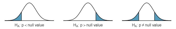
When the alternative claim uses a \(\neq\text{,}\) we call the test a two-sided test, because either extreme provides evidence against \(H_0\text{.}\) When the alternative claim uses a \(\lt\) or a \(>\text{,}\) we call it a one-sided test.
TIP: One-sided and two-sided tests
If the researchers are only interested in showing an increase or a decrease, but not both, use a one-sided test. If the researchers would be interested in any difference from the null value — an increase or decrease — then the test should be two-sided.
Example 5.3.8
For the example of the consultant's complication rate, we knew that her sample complication rate was 0.063, which was lower than the US complication rate of 0.10. Why did we conduct a two-sided hypothesis test for this setting?
Solution
The setting was framed in the context of the consultant being helpful, but what if the consultant actually performed worse than the US complication rate? Would we care? More than ever! Since we care about a finding in either direction, we should run a two-sided test.
Caution: One-sided hypotheses are allowed only before seeing data
After observing data, it is tempting to turn a two-sided test into a one-sided test. Avoid this temptation. Hypotheses must be set up before observing the data. If they are not, the test must be two-sided.
Subsection 5.3.3 Evaluating the hypotheses with a p-value
Example 5.3.9
There were 142 patients in the consultant's sample. If the null claim is true, how many would we expect to have had a complication?
Solution
If the null claim is true, we would expect about 10% of the patients, or about 14.2 to have a complication.
The consultant's complication rate for her 142 clients was 0.063 (\(0.063 \times 142 \approx 9\)). What is the probability that a sample would produce a number of complications this far from the expected value of 14.2, if her true complication rate were 0.10, that is, if \(H_0\) were true? The probability, which is estimated in Figure 5.3.10, is about 0.1754. We call this quantity the p-value.

Finding and interpreting the p-value
When examining a proportion, we find and interpret the p-value according to the nature of the alternative hypothesis.
\(H_A:p \gt p_0\text{.}\) The p-value is the probability of observing a sample proportion as large as we saw in our sample, if the null hypothesis were true. The p-value corresponds to the area in the upper tail.
\(H_A:p \lt p_0\text{.}\) The p-value is the probability of observing a sample proportion as small as we saw in our sample, if the null hypothesis were true. The p-value corresponds to the area in the lower tail.
\(H_A:p \neq p_0\text{.}\) The p-value is the probability of observing a sample proportion as far from the null value as what was observed in the current data set, if the null hypothesis were true. The p-value corresponds to the area in both tails.
When the p-value is small, i.e. less than a previously set threshold, we say the results are statistically significant. This means the data provide such strong evidence against \(H_0\) that we reject the null hypothesis in favor of the alternative hypothesis. The threshold, called the significance level and often represented by \(\alpha\) (the Greek letter alpha ), is typically set to \(\alpha = 0.05\text{,}\) but can vary depending on the field or the application.
Statistical significance
If the p-value is less than the significance level \(\alpha\) (usually 0.05), we say that the result is statistically significant. We reject \(H_0\text{,}\) and we have strong evidence favoring \(H_A\text{.}\)
If the p-value is greater than the significance level \(\alpha\text{,}\) we say that the result is not statistically significant. We do not reject \(H_0\text{,}\) and we do not have strong evidence for \(H_A\text{.}\)
Recall that the null claim is the claim of no difference. If we reject \(H_0\text{,}\) we are asserting that there is a real difference. If we do not reject \(H_0\text{,}\) we are saying that the null claim is reasonable, but it has not been proven.
Guided Practice 5.3.12
Because the p-value is 0.1754, which is larger than the significance level 0.05, we do not reject the null hypothesis. Explain what this means in the context of the problem using plain language. 3 The data do not provide evidence that the consultant's complication rate is significantly lower or higher that the US complication rate of 10%.
Example 5.3.13
In the previous exercise, we did not reject \(H_0\text{.}\) This means that we did not disprove the null claim. Is this equivalent to proving the null claim is true?
Solution
No. We did not prove that the consultant's complication rate is exactly equal to 10%. Recall that the test of hypothesis starts by assuming the null claim is true. That is, the test proceeds as an argument by contradiction. If the null claim is true, there is a 0.1754 chance of seeing sample data as divergent from 10% as we saw in our sample. Because 0.1754 is large, it is within the realm of chance error and we cannot say the null hypothesis is unreasonable. 4 The p-value is actually a conditional probability. It is P(getting data at least as divergent from the null value as we observed \(|\) H\(_0\) is true). It is NOT P( H\(_0\) is true \(|\) we got data this divergent from the null value.
TIP: Double negatives can sometimes be used in statistics
In many statistical explanations, we use double negatives. For instance, we might say that the null hypothesis is not implausible or we failed to reject the null hypothesis. Double negatives are used to communicate that while we are not rejecting a position, we are also not saying that we know it to be true.
Example 5.3.14
Does the conclusion in Guided Practice 5.3.12 ensure that there is no real association between the surgical consultant's work and the risk of complications? Explain.
Solution
No. It is possible that the consultant's work is associated with a lower or higher risk of complications. However, the data did not provide enough information to reject the null hypothesis (the sample was too small).
Example 5.3.15
An experiment was conducted where study participants were randomly divided into two groups. Both were given the opportunity to purchase a DVD, but the one half was reminded that the money, if not spent on the DVD, could be used for other purchases in the future while the other half was not. The half that were reminded that the money could be used on other purchases were 20% less likely to continue with a DVD purchase. We determined that such a large difference would only occur about 1-in-150 times if the reminder actually had no influence on student decision-making. What is the p-value in this study? Was the result statistically significant?
Solution
The p-value was 0.006 (about 1/150). Since the p-value is less than 0.05, the data provide statistically significant evidence that US college students were actually influenced by the reminder.
What's so special about 0.05?
We often use a threshold of 0.05 to determine whether a result is statistically significant. But why 0.05? Maybe we should use a bigger number, or maybe a smaller number. If you're a little puzzled, that probably means you're reading with a critical eye — good job! We've made a video to help clarify why 0.05:
Sometimes it's also a good idea to deviate from the standard. We'll discuss when to choose a threshold different than 0.05 in Subsection 5.3.7.
Statistical inference is the practice of making decisions and conclusions from data in the context of uncertainty. Just as a confidence interval may occasionally fail to capture the true parameter, a test of hypothesis may occasionally lead us to an incorrect conclusion. While a given data set may not always lead us to a correct conclusion, statistical inference gives us tools to control and evaluate how often these errors occur.
Subsection 5.3.4 Calculating the p-value by simulation (special topic)
When conditions for the applying the normal model are met, we use the normal model to find the p-value of a test of hypothesis. In the complication rate example, the distribution is not normal. It is, however, binomial, because we are interested in how many out of 142 patients will have complications.
We could calculate the p-value of this test using binomial probabilities. A more general approach, though, for calculating p-values when the normal model does not apply is to use what is known as simulation. While performing this procedure is outside of the scope of the course, we provide an example here in order to better understand the concept of a p-value.
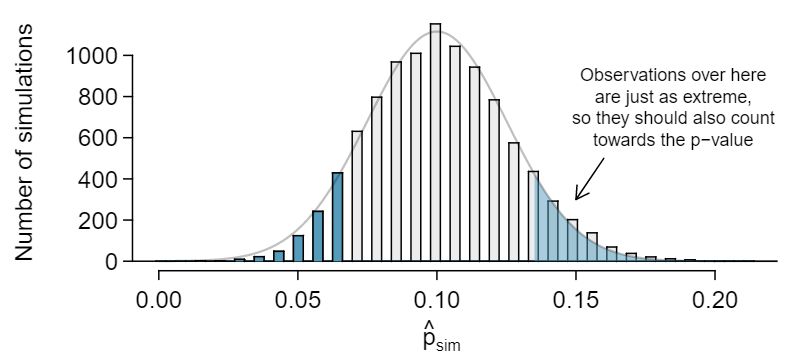
We simulate 142 new patients to see what result might happen if the complication rate really is 0.10. To do this, we could use a deck of cards. Take one red card, nine black cards, and mix them up. If the cards are well-shuffled, drawing the top card is one way of simulating the chance a patient has a complication if the true rate is 0.10: if the card is red, we say the patient had a complication, and if it is black then we say they did not have a complication. If we repeat this process 142 times and compute the proportion of simulated patients with complications, \(\hat{p}_{sim}\text{,}\) then this simulated proportion is exactly a draw from the null distribution.
There were 12 simulated cases with a complication and 130 simulated cases without a complication: \(\hat{p}_{sim} = 12 / 142 = 0.085\text{.}\)
One simulation isn't enough to get a sense of the null distribution, so we repeated the simulation 10,000 times using a computer. Figure 5.3.16 shows the null distribution from these 10,000 simulations. The simulated proportions that are less than or equal to \(\hat{p}=0.063\) are shaded. There were 0.0877 simulated sample proportions with \(\hat{p}_{sim} \leq 0.063\text{,}\) which represents a fraction 0.0877 of our simulations:
\begin{gather*}
\text{ left tail }
= \frac{\text{ Number of observed simulations with } \hat{p}_{sim}\leq\text{ 0.063 } }{10000}
= \frac{877}{10000} = 0.0877
\end{gather*}
However, this is not our p-value! Remember that we are conducting a two-sided test, so we should double the one-tail area to get the p-value: 5 This doubling approach is preferred even when the distribution isn't symmetric, as in this case.
\begin{gather*}
\text{ p-value } = 2 \times \text{ left tail } = 2 \times 0.0877 = 0.1754
\end{gather*}
Subsection 5.3.5 Formal hypothesis testing: a stepwise approach
Carrying out a formal test of hypothesis (AP exam tip)
Follow these seven steps when carrying out a hypothesis test.
State the name of the test being used.
Verify conditions to ensure the standard error estimate is reasonable and the point estimate follows the appropriate distribution and is unbiased.
Write the hypotheses in plain language, then set them up in mathematical notation.
Identify the significance level \(\alpha\text{.}\)
-
Calculate the test statistic, often Z, using an appropriate point estimate of the parameter of interest and its standard error.
\begin{gather*} \text{ test statistic } = \frac{\text{ point estimate } - \text{ null value } }{\text{ SE of estimate } } \end{gather*} Find the p-value, compare it to \(\alpha\text{,}\) and state whether to reject or not reject the null hypothesis.
Write your conclusion in context.
Subsection 5.3.6 Decision errors
The hypothesis testing framework is a very general tool, and we often use it without a second thought. If a person makes a somewhat unbelievable claim, we are initially skeptical. However, if there is sufficient evidence that supports the claim, we set aside our skepticism. The hallmarks of hypothesis testing are also found in the US court system.
Example 5.3.17
A US court considers two possible claims about a defendant: she is either innocent or guilty. If we set these claims up in a hypothesis framework, which would be the null hypothesis and which the alternative?
Solution
The jury considers whether the evidence is so convincing (strong) that there is no reasonable doubt of the person's guilt. That is, the skeptical perspective (null hypothesis) is that the person is innocent until evidence is presented that convinces the jury that the person is guilty (alternative hypothesis). In statistics, our evidence comes in the form of data, and we use the significance level to decide what is beyond a reasonable doubt.
Jurors examine the evidence to see whether it convincingly shows a defendant is guilty. Notice that a jury finds a defendent either guilty or not guilty. They either reject the null claim or they do not reject the null claim. They never prove the null claim, that is, they never find the defendant innocent. If a jury finds a defendant not guilty, this does not necessarily mean the jury is confident in the person's innocence. They are simply not convinced of the alternative that the person is guilty.
This is also the case with hypothesis testing: even if we fail to reject the null hypothesis, we typically do not accept the null hypothesis as truth. Failing to find strong evidence for the alternative hypothesis is not equivalent to providing evidence that the null hypothesis is true.
Hypothesis tests are not flawless. Just think of the court system: innocent people are sometimes wrongly convicted and the guilty sometimes walk free. Similarly, data can point to the wrong conclusion. However, what distinguishes statistical hypothesis tests from a court system is that our framework allows us to quantify and control how often the data lead us to the incorrect conclusion.
There are two competing hypotheses: the null and the alternative. In a hypothesis test, we make a statement about which one might be true, but we might choose incorrectly. There are four possible scenarios in a hypothesis test, which are summarized in Table 5.3.18.
| Test conclusion | |||
| do not reject \(H_0\) | reject \(H_0\) in favor of \(H_A\) | ||
| Truth | \(H_0\) true | okay | Type 1 Error |
| \(H_A\) true | Type 2 Error | okay | |
Type 1 and Type 2 Errors
A Type 1 Error is rejecting the null hypothesis when \(H_0\) is actually true. When we reject the null hypothesis, it is possible that we make a Type 1 Error.
A Type 2 Error is failing to reject the null hypothesis when \(H_A\) is actually true.
Example 5.3.19
In a US court, the defendant is either innocent (\(H_0\)) or guilty (\(H_A\)). What does a Type 1 Error represent in this context? What does a Type 2 Error represent? Table 5.3.18 may be useful.
Solution
If the court makes a Type 1 Error, this means the defendant is innocent (\(H_0\) true) but wrongly convicted. A Type 2 Error means the court failed to reject \(H_0\) (i.e. failed to convict the person) when she was in fact guilty (\(H_A\) true).
Example 5.3.20
How could we reduce the Type 1 Error rate in US courts? What influence would this have on the Type 2 Error rate?
Solution
To lower the Type 1 Error rate, we might raise our standard for conviction from “beyond a reasonable doubt” to “beyond a conceivable doubt” so fewer people would be wrongly convicted. However, this would also make it more difficult to convict the people who are actually guilty, so we would make more Type 2 Errors.
Guided Practice 5.3.21
How could we reduce the Type 2 Error rate in US courts? What influence would this have on the Type 1 Error rate? 6 To lower the Type 2 Error rate, we want to convict more guilty people. We could lower the standards for conviction from “beyond a reasonable doubt” to “beyond a little doubt”. Lowering the bar for guilt will also result in more wrongful convictions, raising the Type 1 Error rate.
Guided Practice 5.3.22
A group of women bring a class action lawsuit that claims discrimination in promotion rates. What would a Type 1 Error represent in this context? 7 We must first identify which is the null hypothesis and which is the alternative. The alternative hypothesis is the one that bears the burden of proof, so the null hypothesis is that there was no discrimination and the alternative hypothesis is that there was discrimination. Making a Type 1 Error in this context would mean that in fact there was no discrimination, even though we concluded that women were discriminated against. Notice that this does not necessarily mean something was wrong with the data or that we made a computational mistake. Sometimes data simply point us to the wrong conclusion, which is why scientific studies are often repeated to check initial findings.
The example and Exercise above provide an important lesson: if we reduce how often we make one type of error, we generally make more of the other type.
Subsection 5.3.7 Choosing a significance level
If \(H_0\) is true, what is the probability that we will incorrectly reject it? In hypothesis testing, we perform calculations under the premise that \(H_0\) is true, and we reject \(H_0\) if the p-value is smaller than the significance level \(\alpha\text{.}\) That is, \(\alpha\) is the probability of making a Type 1 Error. The choice of what to make \(\alpha\) is not arbitrary. It depends on the gravity of the consequences of a Type 1 Error.
Relationship between Type 1 and Type 2 Errors
The probability of a Type 1 Error is called \(\alpha\) and corresponds to the significance level of a test. The probability of a Type 2 Error is called \(\beta\text{.}\) As we make \(\alpha\) smaller, \(\beta\) typically gets larger, and vice versa.
Example 5.3.23
If making a Type 1 Error is especially dangerous or especially costly, should we choose a smaller significance level or a higher significance level?
Solution
Under this scenario, we want to be very cautious about rejecting the null hypothesis, so we demand very strong evidence before we are willing to reject the null hypothesis. Therefore, we want a smaller significance level, maybe \(\alpha = 0.01\text{.}\)
Example 5.3.24
If making a Type 2 Error is especially dangerous or especially costly, should we choose a smaller significance level or a higher significance level?
Solution
We should choose a higher significance level (e.g. 0.10). Here we want to be cautious about failing to reject \(H_0\) when the null is actually false.
TIP: Significance levels should reflect consequences of errors
The significance level selected for a test should reflect the real-world consequences associated with making a Type 1 or Type 2 Error. If a Type 1 Error is very dangerous, make \(\alpha\) smaller.
Subsection 5.3.8 Statistical power of a hypothesis test
When the alternative hypothesis is true, the probability of not making a Type 2 Error is called power. It is common for researchers to perform a power analysis to ensure their study collects enough data to detect the effects they anticipate finding. As you might imagine, if the effect they care about is small or subtle, then if the effect is real, the researchers will need to collect a large sample size in order to have a good chance of detecting the effect. However, if they are interested in large effect, they need not collect as much data.
The Type 2 Error rate \(\beta\) and the magnitude of the error for a point estimate are controlled by the sample size. As the sample size \(n\) goes up, the Type 2 Error rate goes down, and power goes up. Real differences from the null value, even large ones, may be difficult to detect with small samples. However, if we take a very large sample, we might find a statistically significant difference but the magnitude might be so small that it is of no practical value.