
Section 6.3 Testing for goodness of fit using chi-square
¶OpenIntro: Testing for goodness of fit using chi square
In this section, we develop a method for assessing a null model when the data are binned. This technique is commonly used in two circumstances:
Given a sample of cases that can be classified into several groups, determine if the sample is representative of the general population.
Evaluate whether data resemble a particular distribution, such as a normal distribution or a geometric distribution.
Each of these scenarios can be addressed using the same statistical test: a chi-square test.
In the first case, we consider data from a random sample of 275 jurors in a small county. Jurors identified their racial group, as shown in Table 6.3.2, and we would like to determine if these jurors are racially representative of the population. If the jury is representative of the population, then the proportions in the sample should roughly reflect the population of eligible jurors, i.e. registered voters.
| Race | White | Black | Hispanic | Other | Total | ||
| Representation in juries | 205 | 26 | 25 | 19 | 275 | ||
| Registered voters | 0.72 | 0.07 | 0.12 | 0.09 | 1.00 |
While the proportions in the juries do not precisely represent the population proportions, it is unclear whether these data provide convincing evidence that the sample is not representative. If the jurors really were randomly sampled from the registered voters, we might expect small differences due to chance. However, unusually large differences may provide convincing evidence that the juries were not representative.
A second application, assessing the fit of a distribution, is presented at the end of this section. Daily stock returns from the S&P500 for the years 1990-2011 are used to assess whether stock activity each day is independent of the stock's behavior on previous days.
In these problems, we would like to examine all bins simultaneously, not simply compare one or two bins at a time, which will require us to develop a new test statistic.
Subsection 6.3.1 Creating a test statistic for one-way tables
Of the people in the city, 275 served on a jury. If the individuals are randomly selected to serve on a jury, about how many of the 275 people would we expect to be white? How many would we expect to be black?
Solution
About 72% of the population is white, so we would expect about 72% of the jurors to be white: \(0.72\times 275 = 198\text{.}\)
Similarly, we would expect about 7% of the jurors to be black, which would correspond to about \(0.07\times 275 = 19.25\) black jurors.
Guided Practice 6.3.4
Twelve percent of the population is Hispanic and 9% represent other races. How many of the 275 jurors would we expect to be Hispanic or from another race? Answers can be found in Table 6.3.5.
| Race | White | Black | Hispanic | Other | Total | ||
| Observed data | 205 | 26 | 25 | 19 | 275 | ||
| Expected counts | 198 | 19.25 | 33 | 24.75 | 275 | ||
The sample proportion represented from each race among the 275 jurors was not a precise match for any ethnic group. While some sampling variation is expected, we would expect the sample proportions to be fairly similar to the population proportions if there is no bias on juries. We need to test whether the differences are strong enough to provide convincing evidence that the jurors are not a random sample. These ideas can be organized into hypotheses:
\(H_{0}:\) The jurors are a random sample, i.e. there is no racial bias in who serves on a jury, and the observed counts reflect natural sampling fluctuation.
\(H_{A}:\) The jurors are not randomly sampled, i.e. there is racial bias in juror selection.
To evaluate these hypotheses, we quantify how different the observed counts are from the expected counts. Strong evidence for the alternative hypothesis would come in the form of unusually large deviations in the groups from what would be expected based on sampling variation alone.
Subsection 6.3.2 The chi-square test statistic
¶In previous hypothesis tests, we constructed a test statistic of the following form:
\begin{equation*}
Z = \frac{\text{ point estimate } - \text{ null value } }{\text{ SE of point estimate } }
\end{equation*}
This construction was based on (1) identifying the difference between a point estimate and an expected value if the null hypothesis was true, and (2) standardizing that difference using the standard error of the point estimate. These two ideas will help in the construction of an appropriate test statistic for count data.
In this example we have four categories: white, black, hispanic, and other. Because we have four values rather than just one or two, we need a new tool to analyze the data. Our strategy will be to find a test statistic that measures the overall deviation between the observed and the expected counts. We first find the difference between the observed and expected counts for the four groups:
\begin{align*}
\amp \amp \text{ White } \amp \amp \text{ Black } \amp \amp \text{ Hispanic } \amp \amp \text{ Other }\\
\text{ observed - expected } \amp \amp 205-198 \amp \amp 26-19.25
\amp \amp 25-33
\amp \amp 19-24.75
\end{align*}
Next, we square the differences:
\begin{align*}
\amp \amp \text{ White } \amp \amp \text{ Black } \amp \amp \text{ Hispanic } \amp \amp \text{ Other }\\
\text{ (observed - expected) } ^2 \amp \amp (205-198)^2 \amp \amp (26-19.25)^2
\amp \amp (25-33)^2
\amp \amp (19-24.75)^2
\end{align*}
We must standardize each term. To know whether the squared difference is large, we compare it to what was expected. If the expected count was 5, a squared difference of 25 is very large. However, if the expected count was 1,000, a squared difference of 25 is very small. We will divide each of the squared differences by the corresponding expected count.
\begin{align*}
\amp \amp \text{ White } \amp \amp \text{ Black } \amp \amp \text{ Hispanic } \amp \amp \text{ Other }\\
\frac{\text{ (observed - expected) } ^2}{\text{ expected } } \amp \amp \frac{(205-198)^2}{198} \amp \amp \frac{(26-19.25)^2 }{19.25}
\amp \amp \frac{(25-33)^2}{33}
\amp \amp \frac{(19-24.75)^2}{24.75}
\end{align*}
Finally, to arrive at the overall measure of deviation between the observed counts and the expected counts, we add up the terms.
\begin{align*}
X^2 \amp = \sum{\frac{\text{ (observed - expected) } ^2}{\text{ expected } }}\\
\amp = \frac{(205-198)^2}{198}
+ \frac{(26-19.25)^2 }{19.25}
+ \frac{(25-33)^2}{33}
+ \frac{(19-24.75)^2}{24.75}
\end{align*}
We can write an equation for \(X^2\) 1 \(X^2\) chi-square test statistic using the observed counts and expected counts:
\begin{align*}
X^2 \amp =
\frac
{\text{\((\text{ observed count }_1 - \text{ expected count }_1)^2\)} }
{\text{\(\text{ expected count }_1\)} }
+ \dots + \frac
{\text{\((\text{ observed count }_4 - \text{ expected count }_4)^2\)} }
{\text{\(\text{ expected count }_4\)} }
\end{align*}
The final number \(X^2\) summarizes how strongly the observed counts tend to deviate from the null counts.
In Subsection 6.3.4, we will see that if the null hypothesis is true, then \(X^2\) follows a new distribution called a chi-square distribution. Using this distribution, we will be able to obtain a p-value to evaluate whether there appears to be racial bias in the juries for the city we are considering.
Subsection 6.3.3 The chi-square distribution and finding areas
The chi-square distribution is sometimes used to characterize data sets and statistics that are always positive and typically right skewed. Recall the normal distribution had two parameters — mean and standard deviation — that could be used to describe its exact characteristics. The chi-square distribution has just one parameter called degrees of freedom (df), which influences the shape, center, and spread of the distribution.
Guided Practice 6.3.6
Figure 6.3.7 shows three chi-square distributions. (a) How does the center of the distribution change when the degrees of freedom is larger? (b) What about the variability (spread)? (c) How does the shape change? 2 (a) The center becomes larger. If we look carefully, we can see that the center of each distribution is equal to the distribution's degrees of freedom. (b) The variability increases as the degrees of freedom increases. (c) The distribution is very strongly skewed for \(df=2\text{,}\) and then the distributions become more symmetric for the larger degrees of freedom \(df=4\) and \(df=9\text{.}\) In fact, as the degrees of freedom increase, the \(X^2\) distribution approaches a normal distribution.
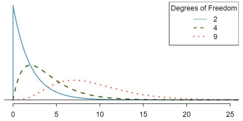
Figure 6.3.7 and Guided Practice 6.3.6 demonstrate three general properties of chi-square distributions as the degrees of freedom increases: the distribution becomes more symmetric, the center moves to the right, and the variability inflates.
Our principal interest in the chi-square distribution is the calculation of p-values, which (as we have seen before) is related to finding the relevant area in the tail of a distribution. To do so, a new table is needed: the chi-square table, partially shown in Table 6.3.8. A more complete table is presented in Appendix D. This table is very similar to the \(t\)-table from Section 7.1 and Section 7.3: we identify a range for the area, and we examine a particular row for distributions with different degrees of freedom. One important difference from the \(t\)-table is that the chi-square table only provides upper tail values.
| Upper tail | 0.3 | 0.2 | 0.1 | 0.05 | 0.02 | 0.01 | 0.005 | 0.001 |
| df 1 | 1.07 | 1.64 | 2.71 | 3.84 | 5.41 | 6.63 | 7.88 | 10.83 |
| df 2 | 2.41 | 3.22 | 4.61 | 5.99 | 7.82 | 9.21 | 10.60 | 13.82 |
| 3 | 3.66 | 4.64 | 6.25 | 7.81 | 9.84 | 11.34 | 12.84 | 16.27 |
| 4 | 4.88 | 5.99 | 7.78 | 9.49 | 11.67 | 13.28 | 14.86 | 18.47 |
| 5 | 6.06 | 7.29 | 9.24 | 11.07 | 13.39 | 15.09 | 16.75 | 20.52 |
| 6 | 7.23 | 8.56 | 10.64 | 12.59 | 15.03 | 16.81 | 18.55 | 22.46 |
| 7 | 8.38 | 9.80 | 12.02 | 14.07 | 16.62 | 18.48 | 20.28 | 24.32 |
Example 6.3.9
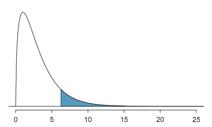
Figure 6.3.11 shows a chi-square distribution with 3 degrees of freedom and an upper shaded tail starting at 6.25. Use Table 6.3.8 to estimate the shaded area.
Solution
This distribution has three degrees of freedom, so only the row with 3 degrees of freedom (df) is relevant. This row has been italicized in the table. Next, we see that the value — 6.25 — falls in the column with upper tail area 0.1. That is, the shaded upper tail of Figure 6.3.11 has area 0.1.
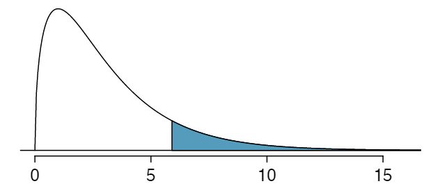
Example 6.3.16
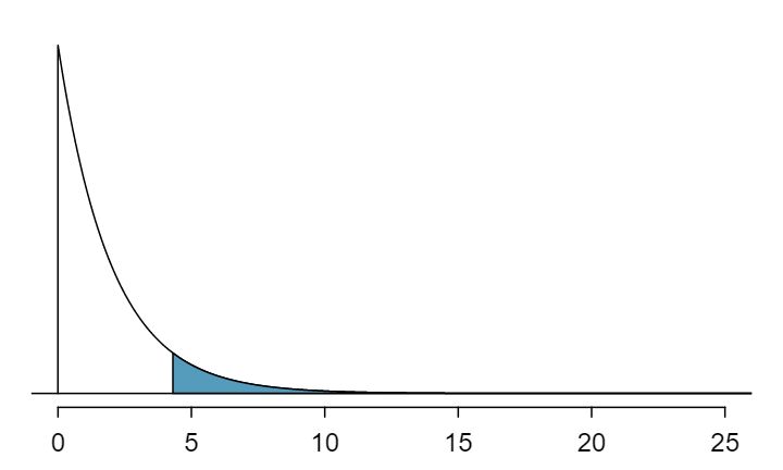
We rarely observe the exact value in the table. For instance, Figure 6.3.10 shows the upper tail of a chi-square distribution with 2 degrees of freedom. The lower bound for this upper tail is at 4.3, which does not fall in Table 6.3.8. Find the approximate tail area.
Solution
The cutoff 4.3 falls between the second and third columns in the 2 degrees of freedom row. Because these columns correspond to tail areas of 0.2 and 0.1, we can be certain that the area shaded in Figure 6.3.10 is between 0.1 and 0.2.
Using a calculator or statistical software allows us to get more precise areas under the chi-square curve than we can get from the table alone.
TI-84: Finding an upper tail area under the chi-square curve
MISSINGVIDEOLINK Use the \(X^2\)cdf command to find areas under the chi-square curve.
Hit
2NDVARS(i.e.DISTR).Choose
8:\(X^2\)cdf.Enter the lower bound, which is generally the chi-square value.
Enter the upper bound. Use a large number, such as 1000.
Enter the degrees of freedom.
Choose
Pasteand hitENTER.
TI-83: Do steps 1-2, then type the lower bound, upper bound, and degrees of freedom separated by commas. e.g. \(X^2\)cdf(5, 1000, 3), and hit ENTER.
Casio fx-9750GII: Finding an upper tail area under the chi-sq. curve
MISSINGVIDEOLINK
Navigate to
STAT(MENUbutton, then hit the2button or selectSTAT).Choose the
DISToption (F5button).Choose the
CHIoption (F3button).Choose the
Ccdoption (F2button).If necessary, select the
Varoption (F2button).Enter the
Lowerbound (generally the chi-square value).Enter the
Upperbound (use a large number, such as 1000).Enter the degrees of freedom,
df.Hit the
EXEbutton.
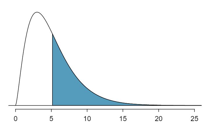
Guided Practice 6.3.17
Figure 6.3.14 shows an upper tail for a chi-square distribution with 5 degrees of freedom and a cutoff of 5.1. Find the tail area using a calculator. 3 Using \(df = 5\) and a lower bound of \(5.1\) for the tail, the upper tail area is 0.4038.
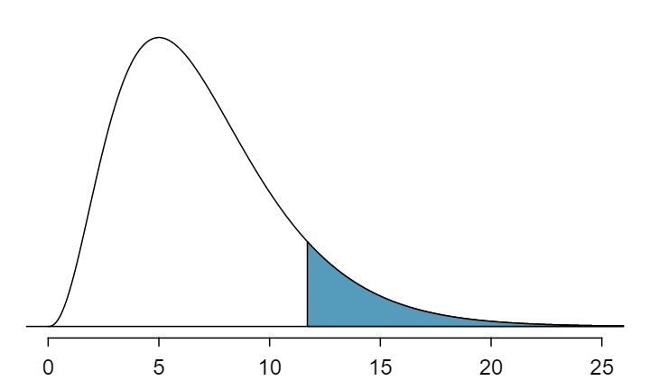
Guided Practice 6.3.18
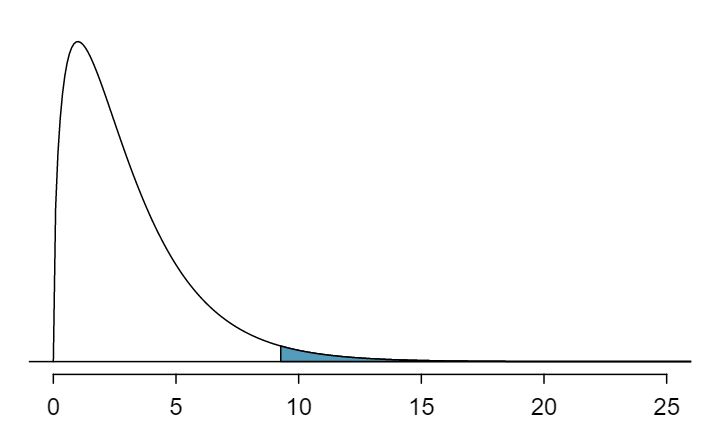
Figure 6.3.15 shows a cutoff of 11.7 on a chi-square distribution with 7 degrees of freedom. Find the area of the upper tail. 4 The area is 0.1109.
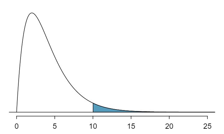
Guided Practice 6.3.19
Figure 6.3.13 shows a cutoff of 10 on a chi-square distribution with 4 degrees of freedom. Find the area of the upper tail. 5 The area is 0.4043.
Guided Practice 6.3.20
Figure 6.3.12 shows a cutoff of 9.21 with a chi-square distribution with 3 df. Find the area of the upper tail. 6 The area is 0.0266.
Subsection 6.3.4 Finding a p-value for a chi-square distribution
¶In Subsection 6.3.2, we identified a new test statistic (\(X^2\)) within the context of assessing whether there was evidence of racial bias in how jurors were sampled. The null hypothesis represented the claim that jurors were randomly sampled and there was no racial bias. The alternative hypothesis was that there was racial bias in how the jurors were sampled.
We determined that a large \(X^2\) value would suggest strong evidence favoring the alternative hypothesis: that there was racial bias. However, we could not quantify what the chance was of observing such a large test statistic (\(X^2=5.89\)) if the null hypothesis actually was true. This is where the chi-square distribution becomes useful. If the null hypothesis was true and there was no racial bias, then \(X^2\) would follow a chi-square distribution, with three degrees of freedom in this case. Under certain conditions, the statistic \(X^2\) follows a chi-square distribution with \(k-1\) degrees of freedom, where \(k\) is the number of bins or categories of the variable.
Example 6.3.21
How many categories were there in the juror example? How many degrees of freedom should be associated with the chi-square distribution used for \(X^2\text{?}\)
Solution
In the jurors example, there were \(k=4\) categories: white, black, Hispanic, and other. According to the rule above, the test statistic \(X^2\) should then follow a chi-square distribution with \(k-1 = 3\) degrees of freedom if \(H_0\) is true.
Just like we checked sample size conditions to use the normal model in earlier sections, we must also check a sample size condition to safely apply the chi-square distribution for \(X^2\text{.}\) Each expected count must be at least 5. In the juror example, the expected counts were 198, 19.25, 33, and 24.75, all easily above 5, so we can apply the chi-square model to the test statistic, \(X^2=5.89\text{.}\)
Example 6.3.22
If the null hypothesis is true, the test statistic \(X^2=5.89\) would be closely associated with a chi-square distribution with three degrees of freedom. Using this distribution and test statistic, identify the p-value and state whether or not there is evidence of racial bias in the juror selection.
Solution
The chi-square distribution and p-value are shown in Figure 6.3.23. Because larger chi-square values correspond to stronger evidence against the null hypothesis, we shade the upper tail to represent the p-value. Using the chi-square table in Appendix D or Table 6.3.8, we can determine that the area is between 0.1 and 0.2. That is, the p-value is larger than 0.1 but smaller than 0.2. Generally we do not reject the null hypothesis with such a large p-value. In other words, the data do not provide convincing evidence of racial bias in the juror selection.
The test that we just carried out regarding jury selection is known as the \(X^2\) goodness of fit test. It is called “goodness of fit” because we test whether or not the proposed or expected distribution is a good fit for the observed data.
Chi-square goodness of fit test for one-way table
Suppose we are to evaluate whether there is convincing evidence that a set of observed counts \(O_1\text{,}\) \(O_2\text{,}\) ..., \(O_k\) in \(k\) categories are unusually different from what might be expected under a null hypothesis. Call the expected counts that are based on the null hypothesis \(E_1\text{,}\) \(E_2\text{,}\) ..., \(E_k\text{.}\) If each expected count is at least 5 and the null hypothesis is true, then the test statistic below follows a chi-square distribution with \(k-1\) degrees of freedom:
\begin{gather*}
X^2 = \frac{(O_1 - E_1)^2}{E_1} + \frac{(O_2 - E_2)^2}{E_2} + \cdots + \frac{(O_k - E_k)^2}{E_k}
\end{gather*}
The p-value for this test statistic is found by looking at the upper tail of this chi-square distribution. We consider the upper tail because larger values of \(X^2\) would provide greater evidence against the null hypothesis.
TIP: Conditions for the chi-square goodness of fit test
There are two conditions that must be checked before performing a chi-square goodness of fit test. If these conditions are not met, this test should not be used.
Simple random sample. The data must be arrived at by taking a simple random sample from the population of interest. The observed counts can then be organized into a list or one-way table.
All Expected Counts at least 5. Each particular scenario (i.e. cell count) must have at least 5 expected cases.
Subsection 6.3.5 Evaluating goodness of fit for a distribution
Goodness of fit test for a one-way table
-
State the name of the test being used.
\(X^2\) goodness of fit test.
-
Verify conditions.
A simple random sample.
All expected counts \(\ge 5\) (calculate and record expected counts).
-
Write the hypotheses in plain language. No mathematical notation is needed for this test.
H\(_0\text{:}\) The distribution of [...] matches [the expected distribution].
H\(_A\text{:}\) The distribution of [....] does not match [the expected distribution]
Identify the significance level \(\alpha\text{.}\)
-
Calculate the test statistic and degrees of freedom.
\begin{align*} X^2 \amp = \sum{\frac{\text{ (observed counts - expected counts) } ^2}{\text{ expected counts } }}\\ df \amp = (\# \text{ of categories } - 1) \end{align*} Find the p-value and compare it to \(\alpha\) to determine whether to reject or not reject \(H_0\text{.}\)
Write the conclusion in the context of the question.
Section 4.3 would be useful background reading for this example, but it is not a prerequisite.
We can apply our new chi-square testing framework to the second problem in this section: evaluating whether a certain statistical model fits a data set. Daily stock returns from the S&P500 for 1990-2011 can be used to assess whether stock activity each day is independent of the stock's behavior on previous days. This sounds like a very complex question, and it is, but a chi-square test can be used to study the problem. We will label each day as Up or Down (D) depending on whether the market was up or down that day. For example, consider the following changes in price, their new labels of up and down, and then the number of days that must be observed before each Up day:
| Change in price | 2.52 | -1.46 | 0.51 | -4.07 | 3.36 | 1.10 | -5.46 | -1.03 | -2.99 | 1.71 | |
| Outcome | Up | D | Up | D | Up | Up | D | D | D | Up | |
| Days to Up | 1 | - | 2 | - | 2 | 1 | - | - | - | 4 |
If the days really are independent, then the number of days until a positive trading day should follow a geometric distribution. The geometric distribution describes the probability of waiting for the \(k^{th}\) trial to observe the first success. Here each up day (Up) represents a success, and down (D) days represent failures. In the data above, it took only one day until the market was up, so the first wait time was 1 day. It took two more days before we observed our next Up trading day, and two more for the third Up day. We would like to determine if these counts (1, 2, 2, 1, 4, and so on) follow the geometric distribution. Table 6.3.24 shows the number of waiting days for a positive trading day during 1990-2011 for the S&P500.
| Days | 1 | 2 | 3 | 4 | 5 | 6 | 7+ | Total | ||
| Observed | 1532 | 760 | 338 | 194 | 74 | 33 | 17 | 2948 |
We consider how many days one must wait until observing an Up day on the S&P500 stock idx. If the stock activity was independent from one day to the next and the probability of a positive trading day was constant, then we would expect this waiting time to follow a geometric distribution. We can organize this into a hypothesis framework:
\(H_0\text{:}\) The stock market being up or down on a given day is independent from all other days. We will consider the number of days that pass until an
Upday is observed. Under this hypothesis, the number of days until anUpday should follow a geometric distribution.\(H_A\text{:}\) The stock market being up or down on a given day is not independent from all other days. Since we know the number of days until an
Upday would follow a geometric distribution under the null, we look for deviations from the geometric distribution, which would support the alternative hypothesis.
There are important implications in our result for stock traders: if information from past trading days is useful in telling what will happen today, that information may provide an advantage over other traders.
We consider data for the S&P500 from 1990 to 2011 and summarize the waiting times in Table 6.3.25 and Figure 6.3.26. The S&P500 was positive on 53.2% of those days.
| Days | 1 | 2 | 3 | 4 | 5 | 6 | 7+ | Total | ||
| Observed | 1532 | 760 | 338 | 194 | 74 | 33 | 17 | 2948 | ||
| Geometric Model | 1569 | 734 | 343 | 161 | 75 | 35 | 31 | 2948 |
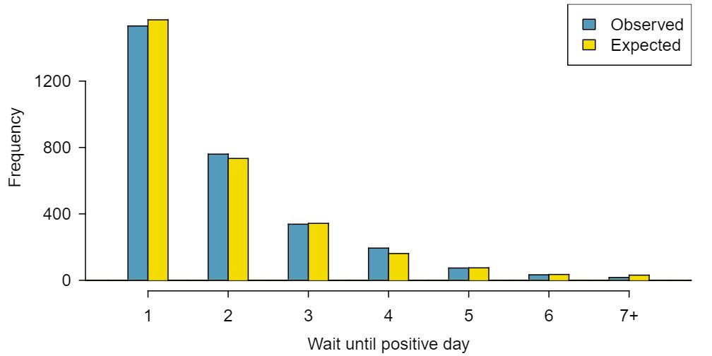
Because applying the chi-square framework requires expected counts to be at least 5, we have binned together all the cases where the waiting time was at least 7 days to ensure each expected count is well above this minimum. The actual data, shown in the Observed row in Table 6.3.25, can be compared to the expected counts from the Geometric Model row. The method for computing expected counts is discussed in Table 6.3.25. In general, the expected counts are determined by (1) identifying the null proportion associated with each bin, then (2) multiplying each null proportion by the total count to obtain the expected counts. That is, this strategy identifies what proportion of the total count we would expect to be in each bin.
Example 6.3.27
Do you notice any unusually large deviations in the graph? Can you tell if these deviations are due to chance just by looking?
Solution
It is not obvious whether differences in the observed counts and the expected counts from the geometric distribution are significantly different. That is, it is not clear whether these deviations might be due to chance or whether they are so strong that the data provide convincing evidence against the null hypothesis. However, we can perform a chi-square test using the counts in Table 6.3.25.
Guided Practice 6.3.28
Table 6.3.25 provides a set of count data for waiting times (\(O_1=1532\text{,}\) \(O_2=760\text{,}\) ...) and expected counts under the geometric distribution (\(E_1=1569\text{,}\) \(E_2=734\text{,}\) ...). Compute the chi-square test statistic, \(X^2\text{.}\) 7 \(X^2=\frac{(1532-1569)^2}{1569} + \frac{(760-734)^2}{734} + \cdots + \frac{(17-31)^2}{31} = 15.08\)
Guided Practice 6.3.29
Because the expected counts are all at least 5, we can safely apply the chi-square distribution to \(X^2\text{.}\) However, how many degrees of freedom should we use? 8 There are \(k=7\) groups, so we use \(df=k-1=6\text{.}\)
Example 6.3.30
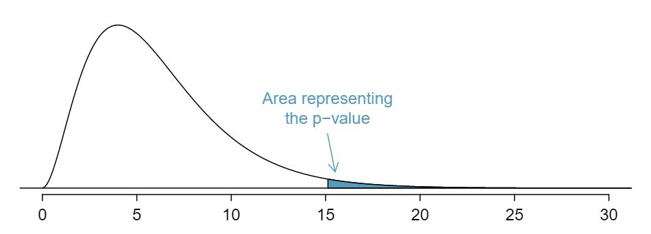
If the observed counts follow the geometric model, then the chi-square test statistic \(X^2=15.08\) would closely follow a chi-square distribution with \(df=6\text{.}\) Using this information, compute a p-value.
Solution
Figure 6.3.31 shows the chi-square distribution, cutoff, and the shaded p-value. If we look up the statistic \(X^2=15.08\) in Appendix D, we find that the p-value is between 0.01 and 0.02. In other words, we have sufficient evidence to reject the notion that the wait times follow a geometric distribution, i.e. trading days are not independent and past days may help predict what the stock market will do today.
Example 6.3.32
In Example 6.3.30, we rejected the null hypothesis that the trading days are independent. Why is this so important?
Solution
Because the data provided strong evidence that the geometric distribution is not appropriate, we reject the claim that trading days are independent. While it is not obvious how to exploit this information, it suggests there are some hidden patterns in the data that could be interesting and possibly useful to a stock trader.
Subsection 6.3.6 Calculator: chi-square goodness of fit test
{\tBoxTitle{MISSINGVIDEOLINK TI-84: Chi-square goodness of fit test} Use STAT, TESTS, \(X^2\)GOF-Test.
Enter the observed counts into list
L1and the expected counts into listL2.Choose
STAT.Right arrow to
TESTS.Down arrow and choose
D:\(X^2\)GOF-Test.Leave
Observed:L1andExpected:L2.Enter the degrees of freedom after
df:Choose
Calculateand hitENTER, which returns:\(X^2\) chi-square test statistic pp-value dfdegrees of freedom
TI-83: Unfortunately the TI-83 does not have this test built in. To carry out the test manually, make list L3 = (L1 - L2)\(^2\) / L2 and do 1-Var-Stats on L3. The sum of L3 will correspond to the value of \(X^2\) for this test.
Casio fx-9750GII: Chi-square goodness of fit test
Navigate to
STAT(MENUbutton, then hit the2button or selectSTAT).Enter the observed counts into a list (e.g.
List 1) and the expected counts into list (e.g.List 2).Choose the
TESToption (F3button).Choose the
CHIoption (F3button).Choose the
GOFoption (F1button).Adjust the
ObservedandExpectedlists to the corresponding list numbers from Step 2.Enter the degrees of freedom,
df.Specify a list where the contributions to the test statistic will be reported using
CNTRB. This list number should be different from the others.Hit the
EXEbutton, which returns\(x^2\) chi-square test statistic pp-value dfdegrees of freedom CNTRBlist showing the test statistic contributions
| Days | 1 | 2 | 3 | 4 | 5 | 6 | 7+ | Total | ||
| Observed | 1532 | 760 | 338 | 194 | 74 | 33 | 17 | 2948 | ||
| Geometric Model | 1569 | 734 | 343 | 161 | 75 | 35 | 31 | 2948 |
Guided Practice 6.3.34
Use the data above and a calculator to find the \(X^2\) statistic, df, and p-value for chi-square goodness of fit test. 9 You should find that \(X^2=15.08\text{,}\) \(df=6\text{,}\) and \(\text{ p-value } =0.0196\text{.}\)