1 Area under the curve, I
What percent of a standard normal distribution \(N(\mu=0, \sigma=1)\) is found in each region? Be sure to draw a graph.
What percent of a standard normal distribution \(N(\mu=0, \sigma=1)\) is found in each region? Be sure to draw a graph.
What percent of a standard normal distribution \(N(\mu=0, \sigma=1)\) is found in each region? Be sure to draw a graph.
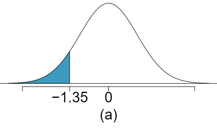
\(Z \gt -1.13\)
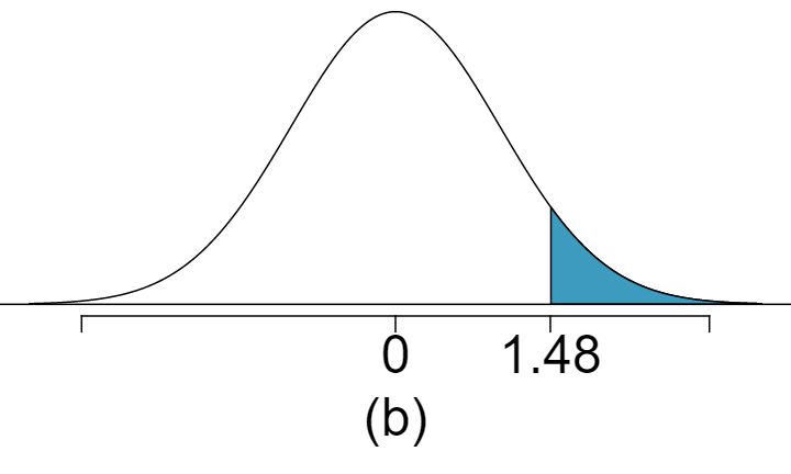
\(Z \lt 0.18\)
\(Z \gt 8\)
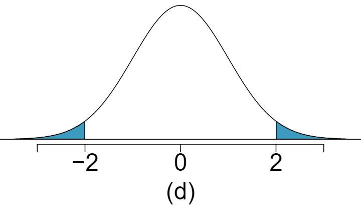
\(|Z| \lt 0.5\)
Sophia who took the Graduate Record Examination (GRE) scored 160 on the Verbal Reasoning section and 157 on the Quantitative Reasoning section. The mean score for Verbal Reasoning section for all test takers was 151 with a standard deviation of 7, and the mean score for the Quantitative Reasoning was 153 with a standard deviation of 7.67. Suppose that both distributions are nearly normal.
Verbal: \(N(\mu = 151, \sigma = 7)\text{,}\) Quant: \(N(\mu = 153, \sigma = 7.67)\text{.}\)
\(Z_{VR} = 1.29\text{,}\) \(Z_{QR} = 0.52\text{.}\)
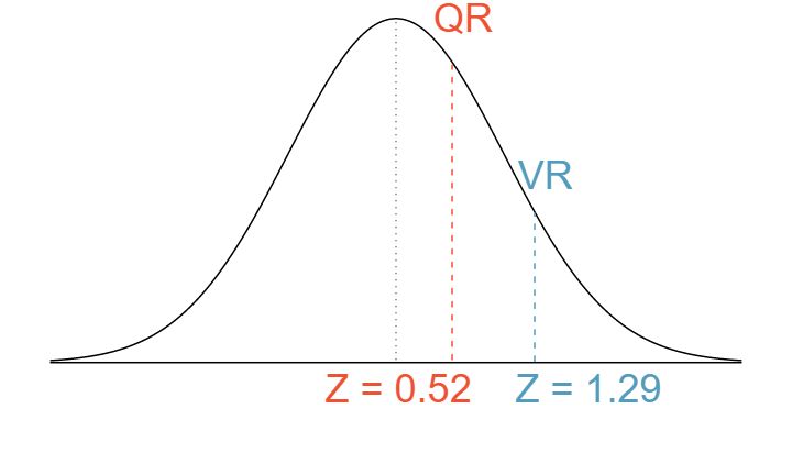
She scored 1.29 standard deviations above the mean on the Verbal Reasoning section and 0.52 standard deviations above the mean on the Quantitative Reasoning section.
She did better on the Verbal Reasoning section since her Z-score on that section was higher.
\(Perc_{VR} = 0.9007 \approx 90\text{,}\) \(Perc_{QR} = 0.6990 \approx 70\text{.}\)
\(100 - 90 = 10\) did better than her on VR, and \(100 - 70 = 30\) did better than her on QR.
Explain why simply comparing raw scores from the two sections could lead to an incorrect conclusion as to which section a student did better on. Answer
We cannot compare the raw scores since they are on different scales. Comparing her percentile scores is more appropriate when comparing her performance to others.
If the distributions of the scores on these exams are not nearly normal, would your answers to parts (b) - (f) change? Explain your reasoning. Answer
Answer to part (b) would not change as Z-scores can be calculated for distributions that are not normal. However, we could not answer parts (d)-(f) since we cannot use the normal probability table to calculate probabilities and percentiles without a normal model.
In triathlons, it is common for racers to be placed into age and gender groups. Friends Leo and Mary both completed the Hermosa Beach Triathlon, where Leo competed in the Men, Ages 30 - 34 group while Mary competed in the Women, Ages 25 - 29 group. Leo completed the race in 1:22:28 (4948 seconds), while Mary completed the race in 1:31:53 (5513 seconds). Obviously Leo finished faster, but they are curious about how they did within their respective groups. Can you help them? Here is some information on the performance of their groups:
The finishing times of the Men, Ages 30 - 34 group has a mean of 4313 seconds with a standard deviation of 583 seconds.
The finishing times of the Women, Ages 25 - 29 group has a mean of 5261 seconds with a standard deviation of 807 seconds.
The distributions of finishing times for both groups are approximately Normal.
Remember: a better performance corresponds to a faster finish.
Write down the short-hand for these two normal distributions.
What are the Z-scores for Leo's and Mary's finishing times? What do these Z-scores tell you?
Did Leo or Mary rank better in their respective groups? Explain your reasoning.
What percent of the triathletes did Leo finish faster than in his group?
What percent of the triathletes did Mary finish faster than in her group?
If the distributions of finishing times are not nearly normal, would your answers to parts (b) - (e) change? Explain your reasoning.
In Exercise 4.6.3 we saw two distributions for GRE scores: \(N(\mu=151, \sigma=7)\) for the verbal part of the exam and \(N(\mu=153, \sigma=7.67)\) for the quantitative part. Use this information to compute each of the following:
\(Z = 0.84\text{,}\) which corresponds to approximately 160 on QR.
\(Z = -0.52\text{,}\) which corresponds to approximately 147 on VR.
In Exercise 4.6.4 we saw two distributions for triathlon times: \(N(\mu=4313, \sigma=583)\) for Men, Ages 30 - 34 and \(N(\mu=5261, \sigma=807)\) for the Women, Ages 25 - 29 group. Times are listed in seconds. Use this information to compute each of the following:
The cutoff time for the fastest 5% of athletes in the men's group, i.e. those who took the shortest 5% of time to finish.
The cutoff time for the slowest 10% of athletes in the women's group.
The average daily high temperature in June in LA is 77°F with a standard deviation of 5 °F. Suppose that the temperatures in June closely follow a normal distribution.
The Capital Asset Pricing Model is a financial model that assumes returns on a portfolio are normally distributed. Suppose a portfolio has an average annual return of 14.7% (i.e. an average gain of 14.7%) with a standard deviation of 33%. A return of 0% means the value of the portfolio doesn't change, a negative return means that the portfolio loses money, and a positive return means that the portfolio gains money.
What percent of years does this portfolio lose money, i.e. have a return less than 0%?
What is the cutoff for the highest 15% of annual returns with this portfolio?
Exercise 4.6.7 states that average daily high temperature in June in LA is 77°F with a standard deviation of 5 °F, and it can be assumed that they to follow a normal distribution. We use the following equation to convert °F (Fahrenheit) to °C (Celsius):
\(N(25, 2.78)\text{.}\)
\(Z = 1.08 \to 0.1401\text{.}\)
The answers are very close because only the units were changed. (The only reason why they are a little different is because 28°C is 82.4 °F, not precisely 83 °F.)
Since \(IQR = Q3 - Q1\text{,}\) we first need to find \(Q3\) and \(Q1\) and take the difference between the two. Remember that \(Q3\) is the \(75^{th}\) and \(Q1\) is the \(25^{th}\) percentile of a distribution. Q1 = 23.13, Q3 = 26.86, IQR = 26.86 - 23.13 = 3.73.
Heights of 10 year olds, regardless of gender, closely follow a normal distribution with mean 55 inches and standard deviation 6 inches.
What is the probability that a randomly chosen 10 year old is shorter than 48 inches?
What is the probability that a randomly chosen 10 year old is between 60 and 65 inches?
If the tallest 10% of the class is considered “very tall”, what is the height cutoff for “very tall”?
The height requirement for Batman the Ride at Six Flags Magic Mountain is 54 inches. What percent of 10 year olds cannot go on this ride?
Suppose a newspaper article states that the distribution of auto insurance premiums for residents of California is approximately normal with a mean of $1,650. The article also states that 25% of California residents pay more than $1,800.
\(Z=0.67\text{.}\)
\(\mu=1650\text{,}\) \(x=1800\text{.}\)
\(0.67 = \frac{1800-1650}{\sigma} \to \sigma=223.88\text{.}\)
The distribution of passenger vehicle speeds traveling on the Interstate 5 Freeway (I-5) in California is nearly normal with a mean of 72.6 miles/hour and a standard deviation of 4.78 miles/hour. 1 S. Johnson and D. Murray. Empirical Analysis of Truck and Automobile Speeds on Rural Interstates: Impact of Posted Speed Limits. In: Transportation Research Board 89th Annual Meeting. 2010.
What percent of passenger vehicles travel slower than 80 miles/hour?
What percent of passenger vehicles travel between 60 and 80 miles/hour?
How fast do the fastest 5% of passenger vehicles travel?
The speed limit on this stretch of the I-5 is 70 miles/hour. Approximate what percentage of the passenger vehicles travel above the speed limit on this stretch of the I-5.
Suppose weights of the checked baggage of airline passengers follow a nearly normal distribution with mean 45 pounds and standard deviation 3.2 pounds. Most airlines charge a fee for baggage that weigh in excess of 50 pounds. Determine what percent of airline passengers incur this fee.
Answer\(Z = 1.56 \to 0.0594\text{,}\) i.e. 6%.
Find the standard deviation of the distribution in the following situations.
MENSA is an organization whose members have IQs in the top 2% of the population. IQs are normally distributed with mean 100, and the minimum IQ score required for admission to MENSA is 132.
Cholesterol levels for women aged 20 to 34 follow an approximately normal distribution with mean 185 milligrams per deciliter (mg/dl). Women with cholesterol levels above 220 mg/dl are considered to have high cholesterol and about 18.5% of women fall into this category.
The textbook you need to buy for your chemistry class is expensive at the college bookstore, so you consider buying it on Ebay instead. A look at past auctions suggest that the prices of that chemistry textbook have an approximately normal distribution with mean $89 and standard deviation $15.
\(Z=0.73 \to 0.2327\text{.}\)
If you are bidding on only one auction and set a low maximum bid price, someone will probably outbid you. If you set a high maximum bid price, you may win the auction but pay more than is necessary. If bidding on more than one auction, and you set your maximum bid price very low, you probably won't win any of the auctions. However, if the maximum bid price is even modestly high, you are likely to win multiple auctions.
An answer roughly equal to the 10th percentile would be reasonable. Regrettably, no percentile cutoff point guarantees beyond any possible event that you win at least one auction. However, you may pick a higher percentile if you want to be more sure of winning an auction.
Answers will vary a little but should correspond to the answer in part (c). We use the 10\(^{th}\) percentile: \(Z = -1.28 \to 69.80\text{.}\)
SAT scores (out of 2400) are distributed normally with a mean of 1500 and a standard deviation of 300. Suppose a school council awards a certificate of excellence to all students who score at least 1900 on the SAT, and suppose we pick one of the recognized students at random. What is the probability this student's score will be at least 2100? (The material covered in Section 3.2 would be useful for this question.)
Below are final exam scores of 20 Introductory Statistics students.
The mean score is 77.7 points. with a standard deviation of 8.44 points. Use this information to determine if the scores approximately follow the 68-95-99.7% Rule.
Answer\(14/20=70\) are within 1 SD. Within 2 SD: \(19/20=95\text{.}\) Within 3 SD: \(20/20 = 100\text{.}\) They follow this rule closely.
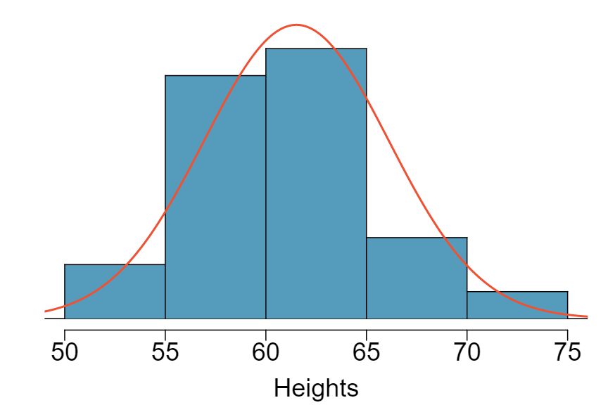
Below are heights of 25 female college students.
The mean height is 61.52 inches with a standard deviation of 4.58 inches. Use this information to determine if the heights approximately follow the 68-95-99.7% Rule.
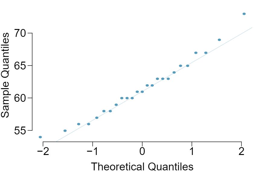
Exercise 4.6.17 lists the final exam scores of 20 Introductory Statistics students. Do these data appear to follow a normal distribution? Explain your reasoning using the graphs provided below.
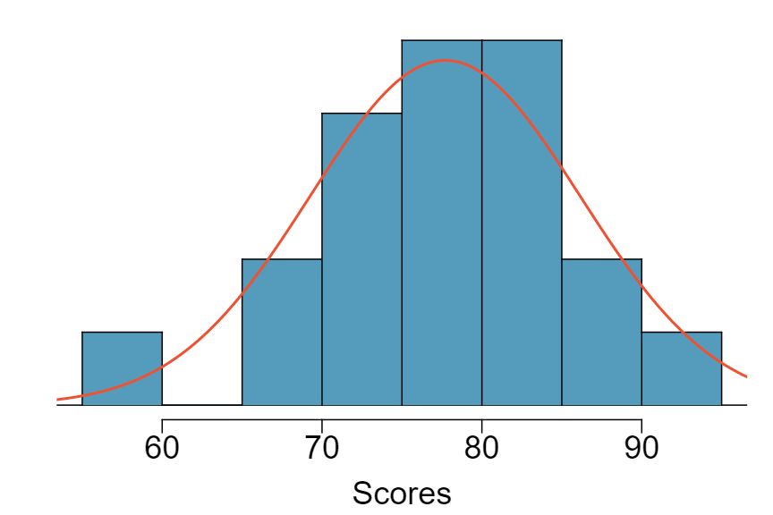
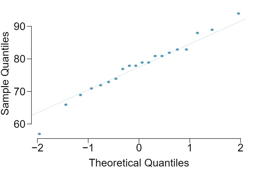
The distribution is unimodal and symmetric. The superimposed normal curve approximates the distribution pretty well. The points on the normal probability plot also follow a relatively straight line. There is one slightly distant observation on the lower end, but it is not extreme. The data appear to be reasonably approximated by the normal distribution.
Exercise 4.6.18 lists the heights of 25 female college students. Do these data appear to follow a normal distribution? Explain your reasoning using the graphs provided below.
Drink pitchers at The Cafe are intended to hold about 64 ounces of lemonade and glasses hold about 12 ounces. However, when the pitchers are filled by a server, they do not always fill it with exactly 64 ounces. There is some variability. Similarly, when they pour out some of the lemonade, they do not pour exactly 12 ounces. The amount of lemonade in a pitcher is normally distributed with mean 64 ounces and standard deviation 1.732 ounces. The amount of lemonade in a glass is normally distributed with mean 12 ounces and standard deviation 1 ounce.
Let X represent the amount of lemonade in the pitcher, Y represent the amount of lemonade in a glass, and W represent the amount left over after. Then, \(\mu_{W} = E(X - Y) = 64 - 12 = 52\)
\(\sigma_{W} = \sqrt{SD(X)^2 + SD(Y)^2} = \sqrt{1.732^2 + 1^2} \approx \sqrt{4} = 2\)
\(P(W \gt 50) = P\left(Z \gt \frac{50 - 52}{2}\right) = P(Z \gt -1) = 1 - 0.1587 = 0.8413\)
Suppose the area that can be painted using a single can of spray paint is slightly variable and follows a nearly normal distribution with a mean of 25 square feet and a standard deviation of 3 square feet. Suppose also that you buy three cans of spray paint.
How much area would you expect to cover with these three cans of spray paint?
What is the standard deviation of the area you expect to cover with these three cans of spray paint?
The area you wanted to cover is 80 square feet. What is the probability that you will be able to cover this entire area with these three cans of spray paint?
In Exercise 4.6.3 we saw two distributions for GRE scores: \(N(\mu=151, \sigma=7)\) for the verbal part of the exam and \(N(\mu=153, \sigma=7.67)\) for the quantitative part. Suppose performance on these two sections is independent. Use this information to compute each of the following:
The combined scores follow a normal distribution with \(\mu_{combined} = 304\) and \(\sigma_{combined} = 10.38\text{.}\) Then, P(combined score \(\gt\) 320) is approximately 0.06.
The combined scores follow a normal distribution with \(\mu_{combined} = 304\) and \(\sigma_{combined} = 10.38\text{.}\) A student who scored better than 90% of other test takers, has \(Z=1.28\text{.}\) Then, we can solve \(1.28 = \frac{x-304}{10.38} \to x\approx 317\text{.}\)
Suppose a restaurant is running a promotion where prices of menu items are determined randomly following some underlying distribution. This means that if you're lucky you can get a basket of fries for $3, or if you're not so lucky you might end up having to pay $10 for the same menu item. The price of basket of fries is drawn from a normal distribution with mean 6 and standard deviation of 2. The price of a fountain drink is drawn from a normal distribution with mean 3 and standard deviation of 1. What is the probability that you pay more than $10 for a dinner consisting of a basket of fries and a fountain drink?
The histogram below shows the distribution of ages of pennies at a bank.
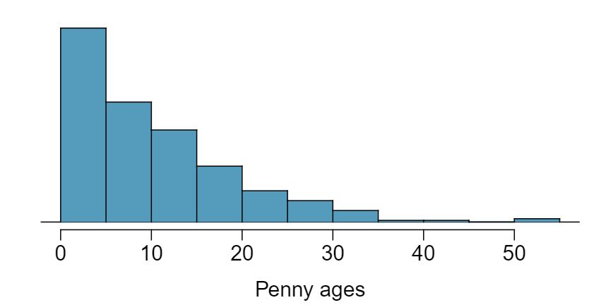
The distribution is unimodal and strongly right skewed with a median between 5 and 10 years old. Ages range from 0 to slightly over 50 years old, and the middle 50% of the distribution is roughly between 5 and 15 years old. There are potential outliers on the higher end.
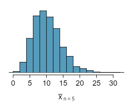
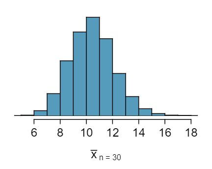
When the sample size is small, the sampling distribution is right skewed, just like the population distribution. As the sample size increases, the sampling distribution gets more unimodal, symmetric, and approaches normality. The variability also decreases. This is consistent with the Central Limit Theorem.
The mean age of the pennies from Exercise 4.6.25 is 10.44 years with a standard deviation of 9.2 years. Using the Central Limit Theorem, calculate the means and standard deviations of the distribution of the mean from random samples of size 5, 30, and 100. Comment on whether the sampling distributions shown in Exercise 4.6.25 agree with the values you compute.
A housing survey was conducted to determine the price of a typical home in Topanga, CA. The mean price of a house was roughly $1.3 million with a standard deviation of $300,000. There were no houses listed below $600,000 but a few houses above $3 million.
Right skewed. There is a long tail on the higher end of the distribution but a much shorter tail on the lower end.
Less than, as the median would be less than the mean in a right skewed distribution.
We should not.
Even though the population distribution is not normal, the conditions for inference are reasonably satisfied, with the possible exception of skew. If the skew isn't very strong (we should ask to see the data), then we can use the Central Limit Theorem to estimate this probability. For now, we'll assume the skew isn't very strong, though the description suggests it is at least moderate to strong. Use \(N(1.3, SD_{\bar{x}} = 0.3/\sqrt{60})\text{:}\) \(Z=2.58\) \(\to\) 0.0049.
It would decrease it by a factor of \(1/\sqrt{2}\text{.}\)
Each year about 1500 students take the introductory statistics course at a large university. This year scores on the final exam are distributed with a median of 74 points, a mean of 70 points, and a standard deviation of 10 points. There are no students who scored above 100 (the maximum score attainable on the final) but a few students scored below 20 points.
Is the distribution of scores on this final exam symmetric, right skewed, or left skewed?
Would you expect most students to have scored above or below 70 points?
Can we calculate the probability that a randomly chosen student scored above 75 using the normal distribution?
What is the probability that the average score for a random sample of 40 students is above 75?
How would cutting the sample size in half affect the standard deviation of the mean?
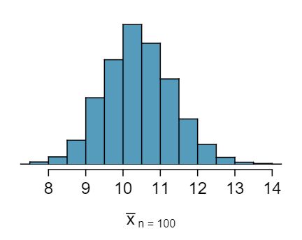
Four plots are presented below. The plot at the top is a distribution for a population. The mean is 10 and the standard deviation is 3. Also shown below is a distribution of (1) a single random sample of 100 values from this population, (2) a distribution of 100 sample means from random samples with size 5, and (3) a distribution of 100 sample means from random samples with size 25. Determine which plot (A, B, or C) is which and explain your reasoning.
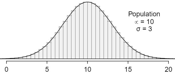
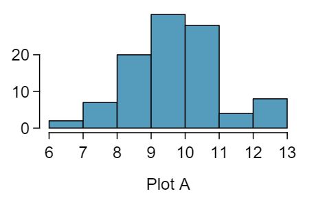
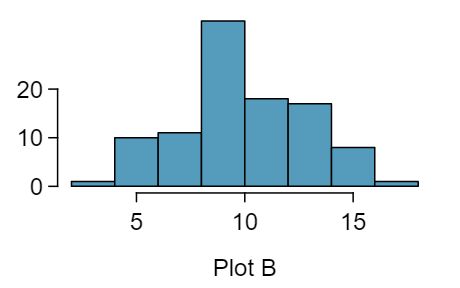
The centers are the same in each plot, and each data set is from a nearly normal distribution (see Subsection 7.1.1), though the histograms may not look very normal since each represents only 100 data points. The only way to tell which plot corresponds to which scenario is to examine the variability of each distribution. Plot B is the most variable, followed by Plot A, then Plot C. This means Plot B will correspond to the original data, Plot A to the sample means with size 5, and Plot C to the sample means with size 25.
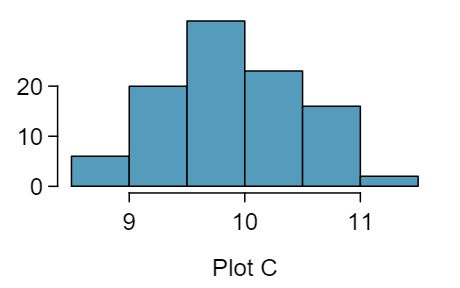
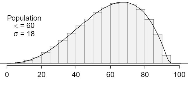
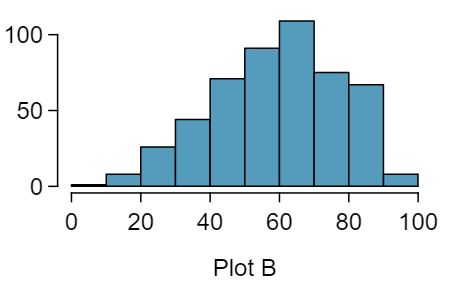
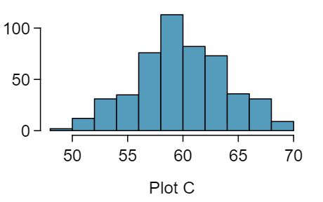
Four plots are presented below. The plot at the top is a distribution for a population. The mean is 60 and the standard deviation is 18. Also shown below is a distribution of (1) a single random sample of 500 values from this population, (2) a distribution of 500 sample means from random samples of each size 18, and (3) a distribution of 500 sample means from random samples of each size 81. Determine which plot (A, B, or C) is which and explain your reasoning.

The distribution of weights of United States pennies is approximately normal with a mean of 2.5 grams and a standard deviation of 0.03 grams.
\(Z=-3.33\) \(\to\) 0.0004.
The population SD is known and the data are nearly normal, so the sample mean will be nearly normal with distribution \(N(\mu, \sigma/\sqrt{n})\text{,}\) i.e. \(N(2.5, 0.0095)\text{.}\)
\(Z=-10.54\) \(\to\) \(\approx0\text{.}\)
See below:
We could not estimate (a) without a nearly normal population distribution. We also could not estimate (c) since the sample size is not sufficient to yield a nearly normal sampling distribution if the population distribution is not nearly normal.
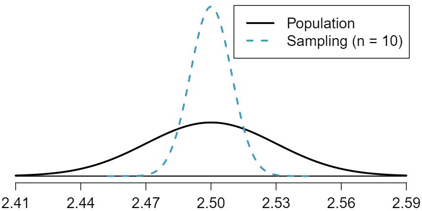
A manufacturer of compact fluorescent light bulbs advertises that the distribution of the lifespans of these light bulbs is nearly normal with a mean of 9,000 hours and a standard deviation of 1,000 hours.
What is the probability that a randomly chosen light bulb lasts more than 10,500 hours?
Describe the distribution of the mean lifespan of 15 light bulbs.
What is the probability that the mean lifespan of 15 randomly chosen light bulbs is more than 10,500 hours?
Sketch the two distributions (population and sampling) on the same scale.
Could you estimate the probabilities from parts (a) and (c) if the lifespans of light bulbs had a skewed distribution?
Suppose an iPod has 3,000 songs. The histogram below shows the distribution of the lengths of these songs. We also know that, for this iPod, the mean length is 3.45 minutes and the standard deviation is 1.63 minutes.
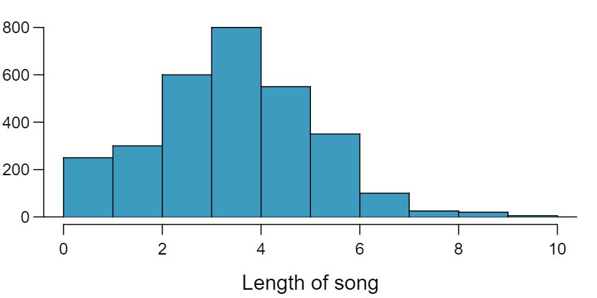
We cannot use the normal model for this calculation, but we can use the histogram. About 500 songs are shown to be longer than 5 minutes, so the probability is about \(500/3000 = 0.167\text{.}\)
Two different answers are reasonable. \(^{Option1}\)Since the population distribution is only slightly skewed to the right, even a small sample size will yield a nearly normal sampling distribution. We also know that the songs are sampled randomly and the sample size is less than 10% of the population, so the length of one song in the sample is independent of another. We are looking for the probability that the total length of 15 songs is more than 60 minutes, which means that the average song should last at least \(60/15 = 4\) minutes. Using \(SD_{\bar{x}}=1.63/\sqrt{15}\text{,}\) \(Z=1.31\) \(\to\) 0.0951. \(^{Option2}\)Since the population distribution is not normal, a small sample size may not be sufficient to yield a nearly normal sampling distribution. Therefore, we cannot estimate the probability using the tools we have learned so far.
We can now be confident that the conditions are satisfied. \(Z = 0.92\) \(\to\) 0.1788.
As described in Exercise 4.6.22, the area that can be painted using a single can of spray paint is slightly variable and follows a nearly normal distribution with a mean of 25 square feet and a standard deviation of 3 square feet.
What is the probability that the area covered by a can of spray paint is more than 27 square feet?
Suppose you want to spray paint an area of 540 square feet using 20 cans of spray paint. On average, how many square feet must each can be able to cover to spray paint all 540 square feet?
What is the probability that you can cover a 540 square feet area using 20 cans of spray paint?
If the area covered by a can of spray paint had a slightly skewed distribution, could you still calculate the probabilities in parts (a) and (c) using the normal distribution?
John is shopping for wireless routers and is overwhelmed by the number of available options. In order to get a feel for the average price, he takes a random sample of 75 routers and finds that the average price for this sample is $75 and the standard deviation is $25.
\(SD_{\bar{x}}=\frac{25}{\sqrt{75}}=2.89\text{.}\)
\(Z=1.73\text{,}\) which indicates that the two values are not unusually distant from each other when accounting for the uncertainty in John's point estimate.
Students are asked to count the number of chocolate chips in 22 cookies for a class activity. The packaging for these cookies claims that there are an average of 20 chocolate chips per cookie with a standard deviation of 4.37 chocolate chips.
Based on this information, about how much variability should they expect to see in the mean number of chocolate chips in random samples of 22 chocolate chip cookies?
What is the probability that a random sample of 22 cookies will have an average less than 14.77 chocolate chips if the companies claim on the packaging is true? Assume that the distribution of chocolate chips in these cookies is approximately normal.
Assume the students got 14.77 as the average in their sample of 22 cookies. Do you have confidence or not in the company's claim that the true average is 20? Explain your reasoning.
Suppose weights of the checked baggage of airline passengers follow a nearly normal distribution with mean 45 pounds and standard deviation 3.2 pounds. What is the probability that the total weight of 10 bags is greater than 460 lbs?
AnswerThis is the same as checking that the average bag weight of the 10 bags is greater than 46 lbs. \(SD_{\bar{x}}=\frac{3.2}{\sqrt{10}}=1.012\text{;}\) \(z= \frac{46-45}{1.012}=0.988\text{;}\) \(P(z \gt 0.988)=0.162=16.2\text{.}\)
Exercise 4.6.24 introduces a promotion at a restaurant where prices of menu items are determined randomly following some underlying distribution. We are told that the price of basket of fries is drawn from a normal distribution with mean 6 and standard deviation of 2. You want to get 5 baskets of fries but you only have $28 in your pocket. What is the probability that you would have enough money to pay for all five baskets of fries?
Determine if each trial can be considered an independent Bernoulli trial for the following situations.
No. The cards are not independent. For example, if the first card is an ace of clubs, that implies the second card cannot be an ace of clubs. Additionally, there are many possible categories, which would need to be simplified.
No. There are six events under consideration. The Bernoulli distribution allows for only two events or categories. Note that rolling a die could be a Bernoulli trial if we simply to two events, e.g. rolling a 6 and not rolling a 6, though specifying such details would be necessary.
In the following situations assume that half of the specified population is male and the other half is female.
Suppose you're sampling from a room with 10 people. What is the probability of sampling two females in a row when sampling with replacement? What is the probability when sampling without replacement?
Now suppose you're sampling from a stadium with 10,000 people. What is the probability of sampling two females in a row when sampling with replacement? What is the probability when sampling without replacement?
We often treat individuals who are sampled from a large population as independent. Using your findings from parts (a) and (b), explain whether or not this assumption is reasonable.
The 2010 American Community Survey estimates that 47.1% of women ages 15 years and over are married. 2 U.S. Census Bureau, 2010 American Community Survey, Marital Status.
\((1-0.471)^2\times0.471 = 0.1318\text{.}\)
\(0.471^3 = 0.1045\text{.}\)
\(\mu = 1/0.471 = 2.12\text{,}\) \(\sigma=\sqrt{2.38} = 1.54\text{.}\)
\(\mu = 1/0.30 = 3.33\text{,}\) \(\sigma=2.79\text{.}\)
When \(p\) is smaller, the event is rarer, meaning the expected number of trials before a success and the standard deviation of the waiting time are higher.
A machine that produces a special type of transistor (a component of computers) has a 2% defective rate. The production is considered a random process where each transistor is independent of the others.
What is the probability that the \(10^{th}\) transistor produced is the first with a defect?
What is the probability that the machine produces no defective transistors in a batch of 100?
On average, how many transistors would you expect to be produced before the first with a defect? What is the standard deviation?
Another machine that also produces transistors has a 5% defective rate where each transistor is produced independent of the others. On average how many transistors would you expect to be produced with this machine before the first with a defect? What is the standard deviation?
Based on your answers to parts (c) and (d), how does increasing the probability of an event affect the mean and standard deviation of the wait time until success?
A husband and wife both have brown eyes but carry genes that make it possible for their children to have brown eyes (probability 0.75), blue eyes (0.125), or green eyes (0.125).
\(0.875^2\times 0.125 = 0.096\text{.}\)
\(\mu=8\text{,}\) \(\sigma=7.48\text{.}\)
Exercise 4.6.12 states that the distribution of speeds of cars traveling on the Interstate 5 Freeway (I-5) in California is nearly normal with a mean of 72.6 miles/hour and a standard deviation of 4.78 miles/hour. The speed limit on this stretch of the I-5 is 70 miles/hour.
A highway patrol officer is hidden on the side of the freeway. What is the probability that 5 cars pass and none are speeding? Assume that the speeds of the cars are independent of each other.
On average, how many cars would the highway patrol officer expect to watch until the first car that is speeding? What is the standard deviation of the number of cars he would expect to watch?
We learned in Exercise 3.7.35 that about 70% of 18-20 year olds consumed alcoholic beverages in 2008. We now consider a random sample of fifty 18-20 year olds.
\(\mu=35\text{,}\) \(\sigma=3.24\text{.}\)
Yes. \(Z=3.09\text{.}\) Since 45 is more than 2 standard deviations from the mean, it would be considered unusual. Note that the normal model is not required to apply this rule of thumb.
Using a normal model: 0.0010. This does indeed appear to be an unusual observation. If using a normal model with a 0.5 correction, the probability would be calculated as 0.0017.
We learned in Exercise 3.7.36 that about 90% of American adults had chickenpox before adulthood. We now consider a random sample of 120 American adults.
How many people in this sample would you expect to have had chickenpox in their childhood? And with what standard deviation?
Would you be surprised if there were 105 people who have had chickenpox in their childhood?
What is the probability that 105 or fewer people in this sample have had chickenpox in their childhood? How does this probability relate to your answer to part (b)?
Suppose a university announced that it admitted 2,500 students for the following year's freshman class. However, the university has dorm room spots for only 1,786 freshman students. If there is a 70% chance that an admitted student will decide to accept the offer and attend this university, what is the approximate probability that the university will not have enough dormitory room spots for the freshman class?
AnswerWant to find the probability that there will be 1,786 or more enrollees. Using the normal: 0.0582. With a 0.5 correction: 0.0559.
Pew Research reported in 2012 that the typical response rate to their surveys is only 9%. If for a particular survey 15,000 households are contacted, what is the probability that at least 1,500 will agree to respond? 3 The Pew Research Center for the People and the Press, Assessing the Representativeness of Public Opinion Surveys, May 15, 2012.
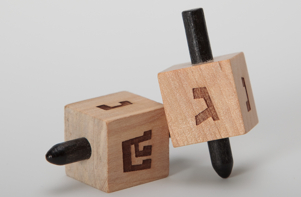
A dreidel is a four-sided spinning top with the Hebrew letters nun, gimel, hei, and shin, one on each side. Each side is equally likely to come up in a single spin of the dreidel. Suppose you spin a dreidel three times. Calculate the probability of getting
\(1-0.75^3 = 0.5781\text{.}\)
0.1406.
0.4219.
\(1-0.25^3=0.9844\text{.}\)
A 2005 Gallup Poll found that 7% of teenagers (ages 13 to 17) suffer from arachnophobia and are extremely afraid of spiders. At a summer camp there are 10 teenagers sleeping in each tent. Assume that these 10 teenagers are independent of each other. 4 Gallup Poll, What Frightens America's Youth?, March 29, 2005.
Calculate the probability that at least one of them suffers from arachnophobia.
Calculate the probability that exactly 2 of them suffer from arachnophobia.
Calculate the probability that at most 1 of them suffers from arachnophobia.
If the camp counselor wants to make sure no more than 1 teenager in each tent is afraid of spiders, does it seem reasonable for him to randomly assign teenagers to tents?
Exercise 4.6.43 introduces a husband and wife with brown eyes who have 0.75 probability of having children with brown eyes, 0.125 probability of having children with blue eyes, and 0.125 probability of having children with green eyes.
Geometric distribution: 0.109.
Binomial: 0.219.
Binomial: 0.137.
\(1-0.875^6=0.551\text{.}\)
Geometric: 0.084.
Using a binomial distribution with \(n = 6\) and \(p=0.75\text{,}\) we see that \(\mu=4.5\text{,}\) \(\sigma=1.06\text{,}\) and \(Z = 2.36\text{.}\) Since this is not within 2 SD, it may be considered unusual.
Sickle cell anemia is a genetic blood disorder where red blood cells lose their flexibility and assume an abnormal, rigid, “sickle” shape, which results in a risk of various complications. If both parents are carriers of the disease, then a child has a 25% chance of having the disease, 50% chance of being a carrier, and 25% chance of neither having the disease nor being a carrier. If two parents who are carriers of the disease have 3 children, what is the probability that
two will have the disease?
none will have the disease?
at least one will neither have the disease nor be a carrier?
the first child with the disease will the be \(3^{rd}\) child?
In the game of roulette, a wheel is spun and you place bets on where it will stop. One popular bet is that it will stop on a red slot; such a bet has an 18/38 chance of winning. If it stops on red, you double the money you bet. If not, you lose the money you bet. Suppose you play 3 times, each time with a $1 bet. Let Y represent the total amount won or lost. Write a probability model for Y.
Answer0 wins (-$3): 0.1458. 1 win (-$1): 0.3936. 2 wins (+$1): 0.3543. 3 wins (+$3): 0.1063.
In a multiple choice quiz there are 5 questions and 4 choices for each question (a, b, c, d). Robin has not studied for the quiz at all, and decides to randomly guess the answers. What is the probability that
the first question she gets right is the \(3^{rd}\) question?
she gets exactly 3 or exactly 4 questions right?
she gets the majority of the questions right?
Suppose the true population proportion were \(p = 0.95\text{.}\) The figure below shows what the distribution of a sample proportion looks like when the sample size is \(n = 20\text{,}\) \(n = 100\text{,}\) and \(n = 500\text{.}\) (a) What does each point (observation) in each of the samples represent? (b) Describe the distribution of the sample proportion, \(\hat{p}\text{.}\) How does the distribution of the sample proportion change as \(n\) becomes larger?
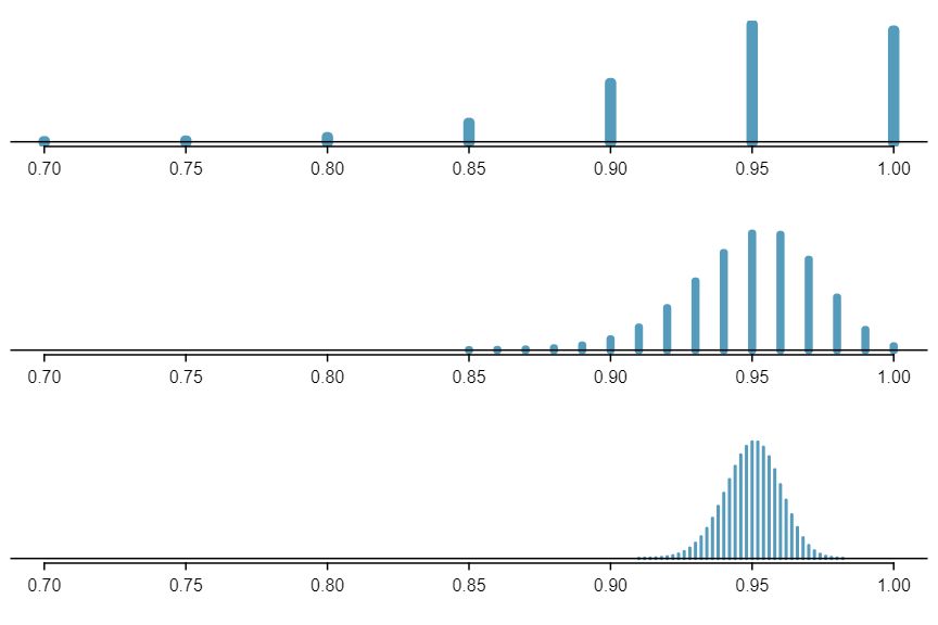
(a) Each observation in each of the distributions represents the sample proportion (\(\hat{p}\)) from samples of size \(n = 20\text{,}\) \(n = 100\text{,}\) and \(n = 500\text{,}\) respectively. (b) The centers for all three distributions are at 0.95, the true population parameter. When \(n\) is small, the distribution is skewed to the left and not smooth. As \(n\) increases, the variability of the distribution (standard deviation) decreases, and the shape of the distribution becomes more unimodal and symmetric.
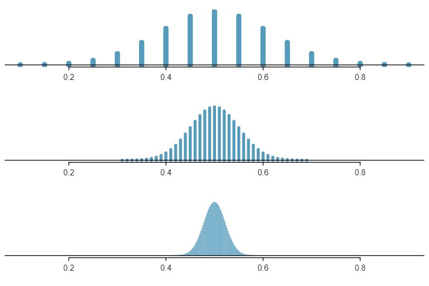
Suppose the true population proportion were \(p = 0.5\text{.}\) The figure below shows what the distribution of a sample proportion looks like when the sample size is \(n = 20\text{,}\) \(n = 100\text{,}\) and \(n = 500\text{.}\) What does each point (observation) in each of the samples represent? Describe how the distribution of the sample proportion, \(\hat{p}\text{,}\) changes as \(n\) becomes larger.
Suppose the true population proportion were \(p = 0.5\) and a researcher takes a simple random sample of size \(n=50\text{.}\)
\(SD_{\hat{p}} = \sqrt{p(1-p) / n} = 0.0707\text{.}\) This describes the typical distance that the sample proportion will deviate from the true proportion, \(p = 0.5\text{.}\)
\(\hat{p}\) approximately follows \(N(0.5, 0.0707)\text{.}\) \(Z = (0.55 - 0.50) / 0.0707 \approx 0.71\text{.}\) This corresponds to an upper tail of about 0.2389. That is, \(P(\hat{p} \gt 0.55) \approx 0.24\text{.}\)
Suppose the true population proportion were \(p = 0.6\) and a researcher takes a simple random sample of size \(n=50\text{.}\)
Find and interpret the standard deviation of the sample proportion \(\hat{p}\text{.}\)
Calculate the probability that the sample proportion will be larger than 0.65 for a random sample of size 50.
It is believed that nearsightedness affects about 8% of all children. We are interested in finding the probability that fewer than 12 out of 200 randomly sampled children will be nearsighted.
First we need to check that the necessary conditions are met. There are \(200 \times 0.08 = 16\) expected successes and \(200 \times (1 - 0.08) = 184\) expected failures, therefore the success-failure condition is met. Then the binomial distribution can be approximated by \(N(\mu = 16, \sigma = 3.84)\text{.}\) \(P(X \lt 12) = P(Z \lt -1.04) = 0.1492\text{.}\)
Since the success-failure condition is met the sampling distribution of \(\hat{p} \sim N(\mu = 0.08, \sigma = 0.0192)\text{.}\) \(P(\hat{p} \lt 0.06) = P(Z \lt -1.04) = 0.1492\text{.}\)
As expected, the two answers are the same.
The 2013 Current Population Survey (CPS) estimates that 22.5% of Mississippians live in poverty, which makes Mississippi the state with the highest poverty rate in the United States. 5 United States Census Bureau. 2013 Current Population Survey. Historical Poverty Tables - People.Web. We are interested in finding out the probability that at least 250 people among a random sample of 1,000 Mississippians live in poverty.
Estimate this probability using the normal approximation to the binomial distribution.
Estimate this probability using the distribution of the sample proportion.
How do your answers from parts (a) and (b) compare?
The 2012 Current Population Survey (CPS) estimates that 38.9% of the people of Hispanic origin in the Unites States are under 21 years old. 6 United States Census Bureau. 2012 Current Population Survey.The Hispanic Population in the United States: 2012. Web. Calculate the probability that at least 35 people among a random sample of 100 Hispanic people living in the United States are under 21 years old.
AnswerFirst we need to check that the necessary conditions are met. There are \(100 \times 0.389 = 38.9\) expected successes and \(100 \times (1 - 0.389) = 61.1\) expected failures, therefore the success-failure condition is met. Calculate using either (1) the normal approximation to the binomial distribution or (2) the sampling distribution of \(\hat{p}\text{.}\) (1) The binomial distribution can be approximated by \(N(\mu = 0.389, \sigma = 4.88)\text{.}\) \(P(X \ge 35) = P(Z \gt -0.80) = 1 - 0.2119 = 0.7881\text{.}\) (2) The sampling distribution of \(\hat{p} \sim N(\mu = 0.389, \sigma = 0.0488)\text{.}\) \(P(\hat{p} \gt 0.35) = P(Z \gt -0.8) = 0.7881\text{.}\)
The Pew Research Center estimates that as of January 2014, 89% of 18-29 year olds in the United States use social networking sites. 7 Pew Research Center, Washington, D.C. Social Networking Fact Sheet, accessed on May 9, 2015. Calculate the probability that at least 95% of 500 randomly sampled 18-29 year olds use social networking sites.