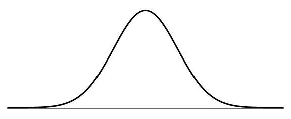
Among all the distributions we see in practice, one is overwhelmingly the most common. The symmetric, unimodal, bell curve is ubiquitous throughout statistics. Indeed it is so common, that people often know it as the normal curve or normal distribution, 1 It is also introduced as the Gaussian distribution after Frederic Gauss, the first person to formalize its mathematical expression. shown in Figure 4.1.2. Variables such as SAT scores and heights of US adult males closely follow the normal distribution.
Normal distribution facts
Many variables are nearly normal, but none are exactly normal. The normal distribution, while never perfect, provides very close approximations for a variety of scenarios. We will use it in data exploration and to solve important problems in statistics.
Subsection4.1.1Normal distribution model
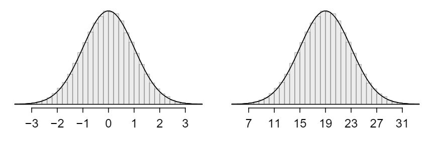
The normal distribution model always describes a symmetric, unimodal, bell-shaped curve. However, these curves can look different depending on the details of the model. Specifically, the normal distribution model can be adjusted using two parameters: mean and standard deviation. As you can probably guess, changing the mean shifts the bell curve to the left or right, while changing the standard deviation stretches or constricts the curve. Figure 4.1.3 shows the normal distribution with mean \(0\) and standard deviation \(1\) in the left panel and the normal distributions with mean \(19\) and standard deviation \(4\) in the right panel. Figure 4.1.4 shows these distributions on the same axis.
Figure4.1.3 Both curves represent the normal distribution, however, they differ in their center and spread. The normal distribution with mean 0 and standard deviation 1 is called the standard normal distribution.
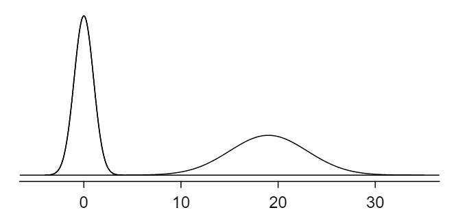
Figure4.1.4 The normal models shown in Figure 4.1.3 but plotted together and on the same scale.
Because the mean and standard deviation describe a normal distribution exactly, they are called the distribution's parameters.
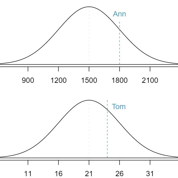
Table 4.1.6 shows the mean and standard deviation for total scores on the SAT and ACT. The distribution of SAT and ACT scores are both nearly normal. Suppose Ann scored 1800 on her SAT and Tom scored 24 on his ACT. Who performed better?
Since the two distributions are on different scales, we use the standard deviation as a guide. Ann is 1 standard deviation above average on the SAT: \(1500 + 300=1800\text{.}\) Tom is 0.6 standard deviations above the mean on the ACT: \(21+0.6\times 5=24\text{.}\) In Figure 4.1.7, we can see that Ann tends to do better with respect to everyone else than Tom did, so her score was better.
SAT
ACT
Mean
1500
21
SD
300
5
Table4.1.6 Mean and standard deviation for the SAT and ACT.
Figure4.1.7 Ann's and Tom's scores shown with the distributions of SAT and ACT scores.
Example 4.1.5 used a standardization technique called a Z-score, a method most commonly employed for nearly normal observations but that may be used with any distribution. The Z-score 2 \(Z\) Z-score, the standardized observation of an observation is defined as the number of standard deviations it falls above or below the mean. If the observation is one standard deviation above the mean, its Z-score is 1. If it is 1.5 standard deviations below the mean, then its Z-score is -1.5. If \(x\) is an observation from a distribution with mean \(\mu\) and standard deviation \(\sigma\text{,}\) we define the Z-score mathematically as
\begin{gather*}
Z = \frac{x-\mu}{\sigma}
\end{gather*}
Using \(\mu_{SAT}=1500\text{,}\) \(\sigma_{SAT}=300\text{,}\) and \(x_{Ann}=1800\text{,}\) we find Ann's Z-score:
The Z-score of an observation is the number of standard deviations it falls above or below the mean. We compute the Z-score for an observation \(x\) that follows a distribution with mean \(\mu\) and standard deviation \(\sigma\) using
\begin{gather*}
Z = \frac{x-\mu}{\sigma}
\end{gather*}
Use Tom's ACT score, 24, along with the ACT mean of 21 and standard deviation of 5 to compute his Z-score. 3 \(Z_{Tom} = \frac{x_{Tom} - \mu_{ACT}}{\sigma_{ACT}} = \frac{24 - 21}{5} = 0.6\)
Observations above the mean always have positive Z-scores while those below the mean have negative Z-scores. If an observation is equal to the mean (e.g. SAT score of 1500), then the Z-score is \(0\text{.}\)
Let \(X\) represent a random variable from a distribution with \(\mu = 3\) and \(\sigma = 2\text{,}\) and suppose we observe \(x=5.19\text{.}\)
Find the Z-score of \(x\text{.}\) 4 Its Z-score is given by \(Z = \frac{x-\mu}{\sigma} = \frac{5.19 - 3}{2} = 2.19/2 = 1.095\text{.}\)
Use the Z-score to determine how many standard deviations above or below the mean \(x\) falls. 5 The observation \(x\) is 1.095 standard deviations above the mean. We know it must be above the mean since \(Z\) is positive.
Head lengths of brushtail possums follow a nearly normal distribution with mean 92.6 mm and standard deviation 3.6 mm. Compute the Z-scores for possums with head lengths of 95.4 mm and 85.8 mm. 6 For \(x_1=95.4\) mm: \(Z_1 = \frac{x_1 - \mu}{\sigma} = \frac{95.4 - 92.6}{3.6} = 0.78\text{.}\) For \(x_2=85.8\) mm: \(Z_2 = \frac{85.8 - 92.6}{3.6} = -1.89\text{.}\)
We can use Z-scores to roughly identify which observations are more unusual than others. One observation \(x_1\) is said to be more unusual than another observation \(x_2\) if the absolute value of its Z-score is larger than the absolute value of the other observation's Z-score: \(|Z_1| \gt |Z_2|\text{.}\) This technique is especially insightful when a distribution is symmetric.
Which of the observations in Guided Practice 4.1.10 is more unusual? 7 Because the absolute value of Z-score for the second observation is larger than that of the first, the second observation has a more unusual head length.
Ann from Example 4.1.5 earned a score of 1800 on her SAT with a corresponding \(Z=1\text{.}\) She would like to know what percentile she falls in among all SAT test-takers.
Ann's percentile is the percentage of people who earned a lower SAT score than Ann. We shade the area representing those individuals in Figure 4.1.13. The total area under the normal curve is always equal to 1, and the proportion of people who scored below Ann on the SAT is equal to the area shaded in Figure 4.1.13: 0.8413. In other words, Ann is in the \(84^{th}\) percentile of SAT takers.
Figure4.1.13 The normal model for SAT scores, shading the area of those individuals who scored below Ann.
We can use the normal model to find percentiles. A normal probability table, which lists Z-scores and corresponding percentiles, can be used to identify a percentile based on the Z-score (and vice versa). Statistical software can also be used.
A normal probability table is given in Appendix B and abbreviated in Table 4.1.15. We use this table to identify the percentile corresponding to any particular Z-score. For instance, the percentile of \(Z=0.43\) is shown in row \(0.4\) and column \(0.03\) in Table 4.1.15: 0.6664, or the \(66.64^{th}\) percentile. Generally, we round \(Z\) to two decimals, identify the proper row in the normal probability table up through the first decimal, and then determine the column representing the second decimal value. The intersection of this row and column is the percentile of the observation.
Figure4.1.14 The area to the left of \(Z\) represents the percentile of the observation.
Second decimal place of \(Z\)
\(Z\)
0.00
0.01
0.02
0.03
0.04
0.05
0.06
0.07
0.08
0.09
0.0
0.5000
0.5040
0.5080
0.5120
0.5160
0.5199
0.5239
0.5279
0.5319
0.5359
0.1
0.5398
0.5438
0.5478
0.5517
0.5557
0.5596
0.5636
0.5675
0.5714
0.5753
0.2
.5793
0.5832
0.5871
0.5910
0.5948
0.5987
0.6026
0.6064
0.6103
0.6141
0.3
0.6179
0.6217
0.6255
0.6293
0.6331
0.6368
0.6406
0.6443
0.6480
0.6517
0.4
0.6554
0.6591
0.6628
0.6664
0.6700
0.6736
0.6772
0.6808
0.6844
0.6879
0.5
0.6915
0.6950
0.6985
0.7019
0.7054
0.7088
0.7123
0.7157
0.7190
0.7224
0.6
0.7257
0.7291
0.7324
0.7357
0.7389
0.7422
0.7454
0.7486
0.7517
0.7549
0.7
0.7580
0.7611
0.7642
0.7673
0.7704
0.7734
0.7764
0.7794
0.7823
0.7852
0.8
0.7881
0.7910
0.7939
0.7967
0.7995
0.8023
0.8051
0.8078
0.8106
0.8133
0.9
0.8159
0.8186
0.8212
0.8238
0.8264
0.8289
0.8315
0.8340
0.8365
0.8389
1.0
0.8413
0.8438
0.8461
0.8485
0.8508
0.8531
0.8554
0.8577
0.8599
0.8621
1.1
0.8643
0.8665
0.8686
0.8708
0.8729
0.8749
0.8770
0.8790
0.8810
0.8830
\(\vdots\)
\(\vdots\)
\(\vdots\)
\(\vdots\)
\(\vdots\)
\(\vdots\)
\(\vdots\)
\(\vdots\)
\(\vdots\)
\(\vdots\)
\(\vdots\)
Table4.1.15 A section of the normal probability table. The percentile for a normal random variable with \(Z=0.43\) has been emphasized, and the percentile closest to 0.8000 has also been emphasized.
We can also find the Z-score associated with a percentile. For example, to identify Z for the \(80^{th}\) percentile, we look for the value closest to 0.8000 in the middle portion of the table: 0.7995. We determine the Z-score for the \(80^{th}\) percentile by combining the row and column Z values: 0.84.
Determine the proportion of SAT test takers who scored better than Ann on the SAT. 8 If 84% had lower scores than Ann, the proportion of people who had better scores must be 16%. (Generally ties are ignored when the normal model, or any other continuous distribution, is used.)
Subsection4.1.4Normal probability examples
Cumulative SAT scores are approximated well by a normal model with mean 1500 and standard deviation 300.
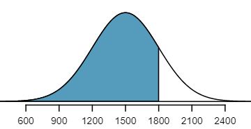
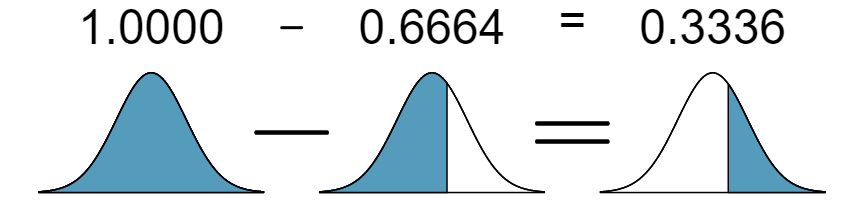
The probability that a randomly selected SAT taker scores at least 1630 on the SAT is equivalent to the proportion of all SAT takers that score at least 1630 on the SAT. First, always draw and label a picture of the normal distribution. (Drawings need not be exact to be useful.) We are interested in the probability that a randomly selected score will be above 1630, so we shade this upper tail:
The picture shows the mean and the values at 2 standard deviations above and below the mean. The simplest way to find the shaded area under the curve makes use of the Z-score of the cutoff value. With \(\mu=1500\text{,}\) \(\sigma=300\text{,}\) and the cutoff value \(x=1630\text{,}\) the Z-score is computed as
We look up the percentile of \(Z=0.43\) in the normal probability table shown in Table 4.1.15 or in Appendix B, which yields 0.6664. However, the percentile describes those who had a Z-score lower than 0.43. To find the area above \(Z=0.43\text{,}\) we compute one minus the area of the lower tail:
The probability that a randomly selected score is at least 1630 on the SAT is 0.3336.
TIP: Always draw a picture first, and find the Z-score second
For any normal probability situation, always always always draw and label the normal curve and shade the area of interest first. The picture will provide an estimate of the probability.
After drawing a figure to represent the situation, identify the Z-score for the observation of interest.
If the probability that a randomly selected score is at least 1630 is 0.3336, what is the probability that the score is less than 1630? Draw the normal curve representing this exercise, shading the lower region instead of the upper one. 9 We found the probability in Example 4.1.17: 0.6664. A picture for this exercise is represented by the shaded area below “0.6664” in Example 4.1.17.
First, a picture is needed. Edward's percentile is the proportion of people who do not get as high as a 1400. These are the scores to the left of 1400.
Identifying the mean \(\mu=1500\text{,}\) the standard deviation \(\sigma=300\text{,}\) and the cutoff for the tail area \(x=1400\) makes it easy to compute the Z-score:
Using the normal probability table, identify the row of \(-0.3\) and column of \(0.03\text{,}\) which corresponds to the probability \(0.3707\text{.}\) Edward is at the \(37^{th}\) percentile.
Use the results of Example 4.1.19 to compute the proportion of SAT takers who did better than Edward. Also draw a new picture. 10 If Edward did better than 37% of SAT takers, then about 63% must have done better than him.
TIP: Areas to the right
The normal probability table in most books gives the area to the left. If you would like the area to the right, first find the area to the left and then subtract this amount from one.
The last several problems have focused on finding the probability or percentile for a particular observation. It is also possible to identify the value corresponding to a particular percentile.
Here, we are given a percentile rather than a Z-score, so we work backwards. As always, first draw the picture.
We want to find the observation that corresponds to the 80th percentile. First, we find the Z-score associated with the 80th percentile using the normal probability table. Looking at Table 4.1.15., we look for the number closest to 0.80 inside the table. The closest number we find is 0.7995 (highlighted). 0.7995 falls on row 0.8 and column 0.04, therefore it corresponds to a Z-score of 0.84. In any normal distribution, a value with a Z-score of 0.84 will be at the 80th percentile. Once we have the Z-score, we work backwards to find x.
Imani scored at the 72nd percentile on the SAT. What was her SAT score? 11 First, draw a picture! The closest percentile in the table to 0.72 is 0.7190, which corresponds to \(Z = 0.58\text{.}\) Next, set up the Z-score formula and solve for \(x\text{:}\) \(0.58 = \frac{x-1500}{300} \rightarrow x = 1674\text{.}\) Imani scored 1674.
Caution: If the data are not nearly normal, don't use a normal table
Before using the normal table, verify that the data or distribution is approximately normal. If it is not, the normal table will give incorrect results. Also, all answers based on normal approximations are approximations and are not exact.
Subsection4.1.5Calculator: finding normal probabilities
Always first sketch a graph: 12 normalcdf gives the result without drawing the graph. To draw the graph, do 2nd VARS, DRAW, 1:ShadeNorm. However, beware of errors caused by other plots that might interfere with this plot.
To find an area under the normal curve using a calculator, first identify a lower bound and an upper bound. Theoretically, we want all of the area to the left of 1.5, so the left endpoint should be -\(\infty\text{.}\) However, the area under the curve is nearly negligible when \(Z\) is smaller than -4, so we will use -5 as the lower bound when not given a lower bound (any other negative number smaller than -5 will also work). Using a lower bound of -5 and an upper bound of 1.5, we get \(P(Z \lt 1.5) = 0.933\text{.}\)
Find the area under the normal curve to right of \(Z=2\text{.}\) 13 Now we want to shade to the right. Therefore our lower bound will be 2 and the upper bound will be +5 (or a number bigger than 5) to get \(P(Z > 2) = 0.023\text{.}\)
Find the area under the normal curve between -1.5 and 1.5. 14 Here we are given both the lower and the upper bound. Lower bound is -1.5 and upper bound is 1.5. The area under the normal curve between -1.5 and 1.5 = \(P(-1.5 \lt Z \lt 1.5) = 0.866\text{.}\)
TI-84: Find a Z-score that corresponds to a percentile
MISSINGVIDEOLINK Use 2NDVARS, invNorm to find the Z-score that corresponds to a given percentile.
Choose 2NDVARS (i.e. DISTR).
Choose 3:invNorm.
Let Area be the percentile as a decimal (the area to the left of desired Z-score).
Leave \(\mu\) as 0 and \(\sigma\) as 1.
Down arrow, choose Paste, and hit ENTER.
TI-83: Do steps 1-2, then enter the percentile as a decimal, e.g. invNorm(0.40) then hit ENTER.
Casio fx-9750GII: Find a Z-score that corresponds to a percentile
MISSINGVIDEOLINK
Navigate to STAT (MENU, then hit 2).
Select DIST (F5), then NORM (F1), and then InvN (F3).
If needed, set Data to Variable (Var option, which is F2).
Decide which tail area to use (Tail), the tail area (Area), and then enter the \(\sigma\) and \(\mu\) values.
Letting Area be 0.40, a calculator gives -0.253. This means that \(Z = -0.253\) corresponds to the 40th percentile, that is, \(P(Z \lt -0.253) = 0.40\text{.}\)
Find the Z-score such that 20 percent of the area is to the right of that Z-score. 15 If 20% of the area is the right, then 80% of the area is to the left. Letting area be 0.80, we get \(Z = 0.841\text{.}\)
In a large study of birth weight of newborns, the weights of 23,419 newborn boys were recorded. 16 www.biomedcentral.com/1471-2393/8/5 The distribution of weights was approximately normal with a mean of 7.44 lbs (3376 grams) and a standard deviation of 1.33 lbs (603 grams). The government classifies a newborn as having low birth weight if the weight is less than 5.5 pounds. What percent of these newborns had a low birth weight?
We find an area under the normal curve between -5 (or a number smaller than -5, e.g. -10) and a Z-score that we will calculate. There is no need to write calculator commands in a solution. Instead, continue to use standard statistical notation.
Approximately what percent of these babies weighed greater than 10 pounds? 17 \(Z=\frac{10-7.44}{1.33}=1.925\text{.}\) Using a lower bound of 2 and an upper bound of 5, we get \(P(Z \gt 1.925) = 0.027\text{.}\) Approximately 2.7% of the newborns weighed over 10 pounds.
Approximately how many of these newborns weighed greater than 10 pounds? 18 Approximately 2.7% of the newborns weighed over 10 pounds. Because there were 23,419 of them, about \(0.027 \times 23419 \approx 632\) weighed greater than 10 pounds.
How much would a newborn have to weigh in order to be at the 90th percentile among this group? 19 Because we have the percentile, this is the inverse problem. To get the Z-score, use the inverse normal option with 0.90 to get \(Z = 1.28\text{.}\) Then solve for \(x\) in \(1.28 = \frac{x - 7.44}{1.33}\) to get \(x = 9.15\text{.}\) To be at the 90th percentile among this group, a newborn would have to weigh 9.15 pounds.
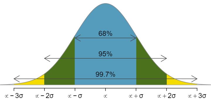
Subsection4.1.668-95-99.7 rule
Here, we present a useful rule of thumb for the probability of falling within 1, 2, and 3 standard deviations of the mean in the normal distribution. This will be useful in a wide range of practical settings, especially when trying to make a quick estimate without a calculator or Z table.
Figure4.1.32 Probabilities for falling within 1, 2, and 3 standard deviations of the mean in a normal distribution.
Use the Z table to confirm that about 68%, 95%, and 99.7% of observations fall within 1, 2, and 3, standard deviations of the mean in the normal distribution, respectively. For instance, first find the area that falls between \(Z=-1\) and \(Z=1\text{,}\) which should have an area of about 0.68. Similarly there should be an area of about 0.95 between \(Z=-2\) and \(Z=2\text{.}\) 20 First draw the pictures. To find the area between \(Z=-1\) and \(Z=1\text{,}\) use the normal probability table to determine the areas below \(Z=-1\) and above \(Z=1\text{.}\) Next verify the area between \(Z=-1\) and \(Z=1\) is about 0.68. Repeat this for \(Z=-2\) to \(Z=2\) and also for \(Z=-3\) to \(Z=3\text{.}\)
It is possible for a normal random variable to fall 4, 5, or even more standard deviations from the mean. However, these occurrences are very rare if the data are nearly normal. The probability of being further than 4 standard deviations from the mean is about 1-in-15,000. For 5 and 6 standard deviations, it is about 1-in-2 million and 1-in-500 million, respectively.
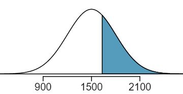
SAT scores closely follow the normal model with mean \(\mu = 1500\) and standard deviation \(\sigma = 300\text{.}\)
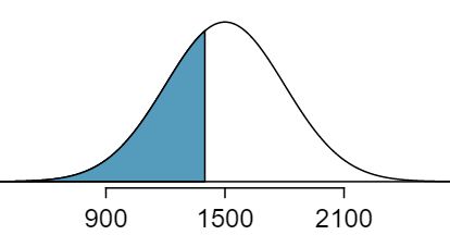
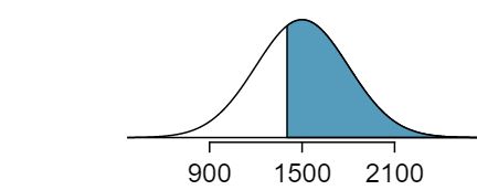
About what percent of test takers score 900 to 2100? 21 900 and 2100 represent two standard deviations above and below the mean, which means about 95% of test takers will score between 900 and 2100.
What percent score between 1500 and 2100? 22 Since the normal model is symmetric, then half of the test takers from part (a) (\(\frac{95\%}{2} = 47.5\%\) of all test takers) will score 900 to 1500 while 47.5% score between 1500 and 2100.
Subsection4.1.7Evaluating the normal approximation
It is important to remember normality is always an approximation. Testing the appropriateness of the normal assumption is a key step in many data analyses.
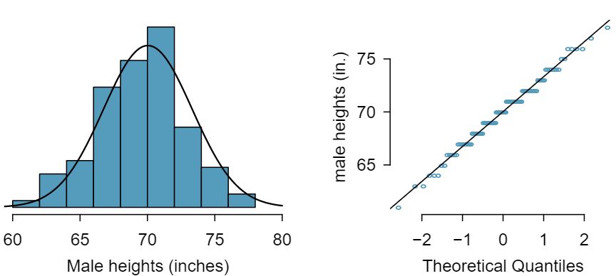
The distribution of heights of US males is well approximated by the normal model. We are interested in proceeding under the assumption that the data are normally distributed, but first we must check to see if this is reasonable.
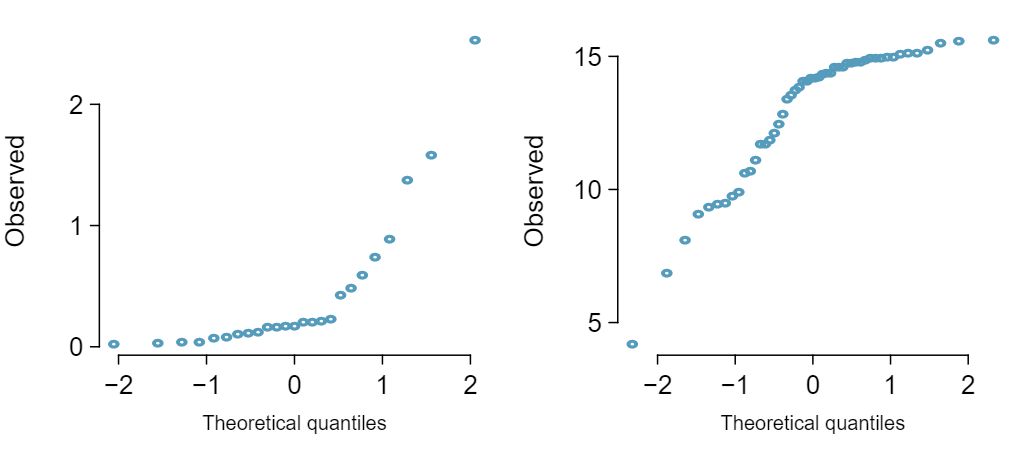
There are two visual methods for checking the assumption of normality that can be implemented and interpreted quickly. The first is a simple histogram with the best fitting normal curve overlaid on the plot, as shown in the left panel of Figure 4.1.35. The sample mean \(\bar{x}\) and standard deviation \(s\) are used as the parameters of the best fitting normal curve. The closer this curve fits the histogram, the more reasonable the normal model assumption. Another more common method is examining a normal probability plot, 23 Also commonly called a quantile-quantile plot. shown in the right panel of Figure 4.1.35. The closer the points are to a perfect straight line, the more confident we can be that the data follow the normal model.
Figure4.1.35 A sample of 100 male heights. The observations are rounded to the nearest whole inch, explaining why the points appear to jump in increments in the normal probability plot.
Three data sets of 40, 100, and 400 samples were simulated from a normal distribution, and the histograms and normal probability plots of the data sets are shown in Figure 4.1.37. These will provide a benchmark for what to look for in plots of real data.
The left panels show the histogram (top) and normal probability plot (bottom) for the simulated data set with 40 observations. The data set is too small to really see clear structure in the histogram. The normal probability plot also reflects this, where there are some deviations from the line. However, these deviations are not strong.
The middle panels show diagnostic plots for the data set with 100 simulated observations. The histogram shows more normality and the normal probability plot shows a better fit. While there is one observation that deviates noticeably from the line, it is not particularly extreme.
The data set with 400 observations has a histogram that greatly resembles the normal distribution, while the normal probability plot is nearly a perfect straight line. Again in the normal probability plot there is one observation (the largest) that deviates slightly from the line. If that observation had deviated 3 times further from the line, it would be of much greater concern in a real data set. Apparent outliers can occur in normally distributed data but they are rare.
Notice the histograms look more normal as the sample size increases, and the normal probability plot becomes straighter and more stable.
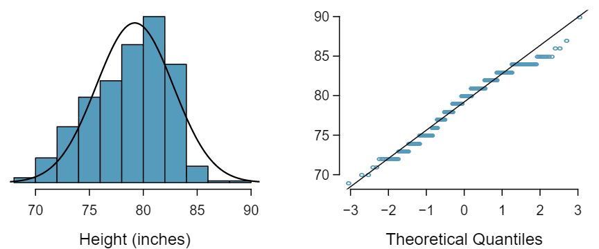
Are NBA player heights normally distributed? Consider all 435 NBA players from the 2008-9 season presented in Figure 4.1.39. 24 These data were collected from www.nba.com.
We first create a histogram and normal probability plot of the NBA player heights. The histogram in the left panel is slightly left skewed, which contrasts with the symmetric normal distribution. The points in the normal probability plot do not appear to closely follow a straight line but show what appears to be a “wave”. We can compare these characteristics to the sample of 400 normally distributed observations in Example 4.1.36 and see that they represent much stronger deviations from the normal model. NBA player heights do not appear to come from a normal distribution.
Figure4.1.39 Histogram and normal probability plot for the NBA heights from the 2008-9 season.
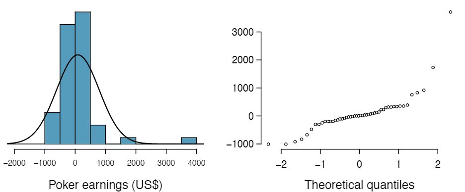
Can we approximate poker winnings by a normal distribution? We consider the poker winnings of an individual over 50 days. A histogram and normal probability plot of these data are shown in Figure 4.1.41.
The data are very strongly right skewed in the histogram, which corresponds to the very strong deviations on the upper right component of the normal probability plot. If we compare these results to the sample of 40 normal observations in Example 4.1.36, it is apparent that these data show very strong deviations from the normal model.
Figure4.1.41 A histogram of poker data with the best fitting normal plot and a normal probability plot.
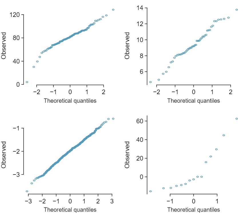
Determine which data sets represented in Figure 4.1.43 plausibly come from a nearly normal distribution. Are you confident in all of your conclusions? There are 100 (top left), 50 (top right), 500 (bottom left), and 15 points (bottom right) in the four plots. 25 Answers may vary a little. The top-left plot shows some deviations in the smallest values in the data set; specifically, the left tail of the data set has some outliers we should be wary of. The top-right and bottom-left plots do not show any obvious or extreme deviations from the lines for their respective sample sizes, so a normal model would be reasonable for these data sets. The bottom-right plot has a consistent curvature that suggests it is not from the normal distribution. If we examine just the vertical coordinates of these observations, we see that there is a lot of data between -20 and 0, and then about five observations scattered between 0 and 70. This describes a distribution that has a strong right skew.
Figure 4.1.45 shows normal probability plots for two distributions that are skewed. One distribution is skewed to the low end (left skewed) and the other to the high end (right skewed). Which is which? 26 Examine where the points fall along the vertical axis. In the first plot, most points are near the low end with fewer observations scattered along the high end; this describes a distribution that is skewed to the high end. The second plot shows the opposite features, and this distribution is skewed to the low end.
We have seen that many distributions are approximately normal. The sum and the difference of normally distributed variables is also normal. While we cannot prove this here, the usefulness of it is seen in the following example.
Three friends are playing a cooperative video game in which they have to complete a puzzle as fast as possible. Assume that the individual times of the 3 friends are independent of each other. The individual times of the friends in similar puzzles are approximately normally distributed with the following means and standard deviations.
Mean
SD
Friend 1
5.6
0.11
Friend 2
5.8
0.13
Friend 3
6.1
0.12
To advance to the next level of the game, the friends' total time must not exceed 17.1 minutes. What is the probability that they will advance to the next level?
Because each friend's time is approximately normally distributed, the sum of their times is also approximately normally distributed. We will do a normal approximation, but first we need to find the mean and standard deviation of the sum. We learned how to do this in Section 3.5.
Let the three friends be labeled \(X\text{,}\) \(Y\text{,}\) \(Z\text{.}\) We want \(P(X + Y + Z \lt 17.1)\text{.}\) The mean and standard deviation of the sum of \(X\text{,}\) \(Y\text{,}\) and \(Z\) is given by:
\begin{align*}
Z \amp = \frac{x_{sum}-\mu_{sum}}{\sigma_{sum}}\\
\amp =\frac{17.1-17.5}{0.208}\\
\amp =-1.92
\end{align*}
Finally, we want the probability that the sum is less than 17.5, so we shade the area to the left of \(Z = -1.92\text{.}\) Using the normal table or a calculator, we get
What is the probability that Friend 2 will complete the puzzle with a faster time than Friend 1? Hint: find \(P(Y \lt X)\text{,}\) or \(P(Y - X \lt 0)\text{.}\) 27 First find the mean and standard deviation of \(Y - X\text{.}\) The mean of \(Y - X\) is \(\mu_{Y-X} = 5.8 - 5.6 = 0.2\text{.}\) The standard deviation is \(SD_{Y-X}=\sqrt{(0.13)^2+(0.11)^2}=0.170\text{.}\) Then \(Z=\frac{0-0.2}{0.170}=-1.18\) and \(P(Z \lt -1.18)= .119\text{.}\) There is an 11.9% chance that Friend 2 will complete the puzzle with a faster time than Friend 1.