
Section 9.1 Review of Graphing
¶Objectives: PCC Course Content and Outcome Guide
This section is a short review of the basics of graphing. The topics here are introduced in Sections 3.1 and 3.2 from Part I. Here we only briefly remind readers of the basics to warm up for the graphing topics in the rest of this chapter. Some readers may benefit from turning to those earlier sections instead of reviewing from this section.
Subsection 9.1.1 Cartesian Coordinates
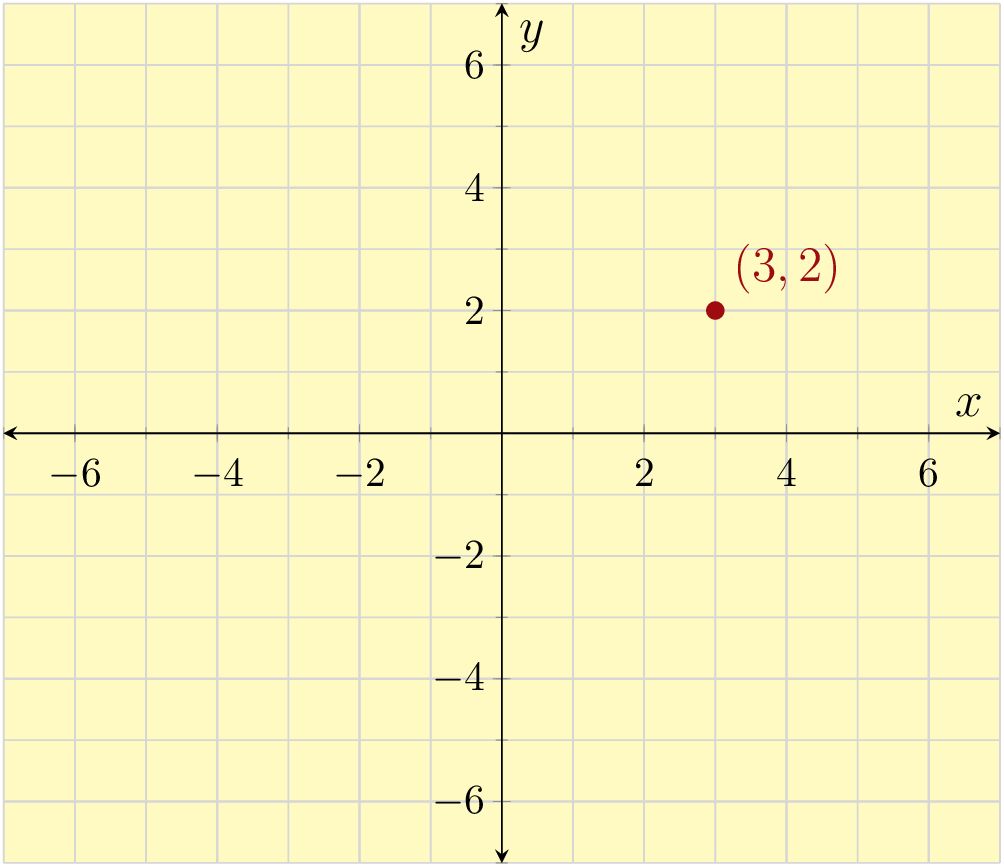
A Cartesian coordinate system is usually represented as a graph where there are two “axes” (straight lines extending infinitely), one horizontal and one vertical. The horizontal axis is usually labeled “\(x\)”, and the vertical axis is usually labeled “\(y\)”. The scale marks on the axes are used to define locations on the plane that they span. An address is a pair of “coordinates” written as in this example: \((3,2)\text{.}\) The first coordinate tells you where the location is with respect to the horizontal axis, and the second coordinate tells you a location with respect to the vertical axis. The point \((3,2)\) is marked in Figure 9.1.2.

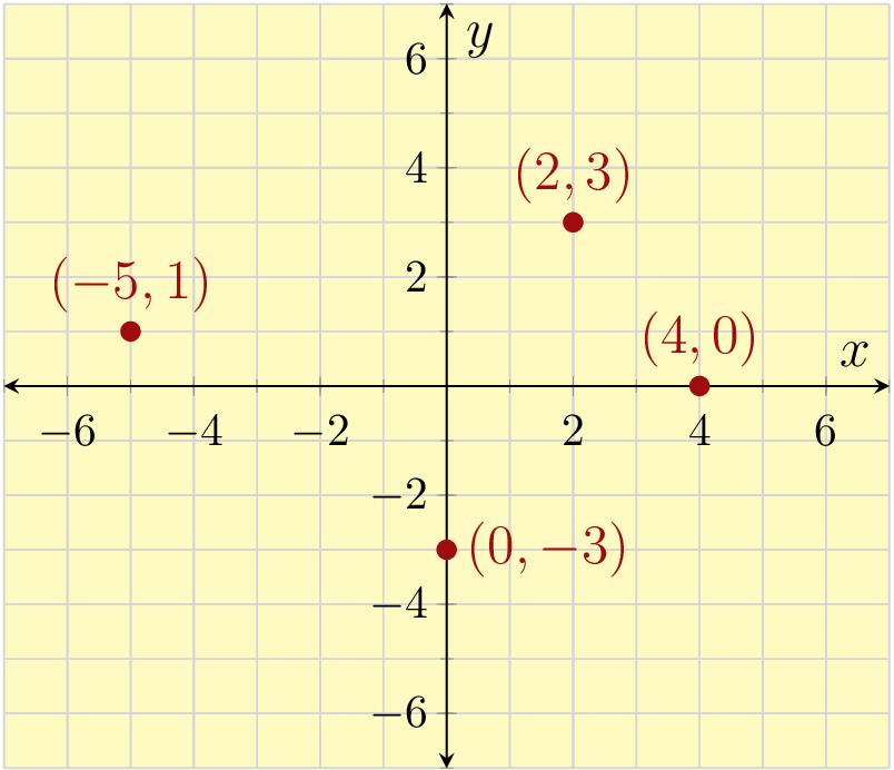
Example 9.1.3.
On paper, sketch a Cartesian coordinate system with the axes scaled using regularly spaced ticks and labels, and then plot the following points: \((2,3),(-5,1),(0,-3),(4,0)\text{.}\)

Subsection 9.1.2 Graphing Equations by Plotting Points
When you have an equation in the form
it suggests that we could substitute in different values for \(x\) and get back different values for \(y\text{.}\) Pairing these \(x\)- and \(y\)-values together, we can plot points and create a “graph” of the equation. Creating a graph of a given equation in \(x\) and \(y\) is the basic objective of this section. Sometimes the equation has special features that give you a shortcut for creating a graph, for example as discussed in Section 3.5. However, here we want to focus on the universal approach of just substituting in values for \(x\) and seeing what comes out.
Example 9.1.5.
Rheema helped plant a lovely Douglas Fir in a local park volunteering with Portland's Friends of Trees 1 friendsoftrees.org/. The tree they planted was 4 ft tall when they planted it. Rheema watched the tree grow over the next few years and noticed that every year, the tree grew about 1.5 ft. So, the height of the tree can be found by using the formula \(y=1.5x+4\text{,}\) where \(x\)-values represent the number of years since the tree was planted. Let's make a graph of this equation by making a table of values. The most straightforward method to graph any equation is to build a table of \(x\)- and \(y\)-values, and then plot the points.
| \(x\) | \(y=1.5x+4\) | Point | Interpretation |
| \(0\) | \(1.5(0)+4\) \({}=4\) |
\((0,4)\) | When the tree was planted, the tree was 4 ft tall. |
| \(2\) | \(1.5(2)+4\) \({}=7\) |
\((2,7)\) | Two years after tree was planted, the tree was 7 ft tall. |
| \(4\) | \(1.5(4)+4\) \({}=10\) |
\((4,10)\) | Four years after tree was planted, the tree was 10 ft tall. |
| \(6\) | \(1.5(6)+4\) \({}=13\) |
\((6,13)\) | Six years after tree was planted, the tree was 13 ft tall. |
| \(8\) | \(1.5(8)+4\) \({}=16\) |
\((8,16)\) | Eight years after tree was planted, the tree was 16 ft tall. |

Example 9.1.8.
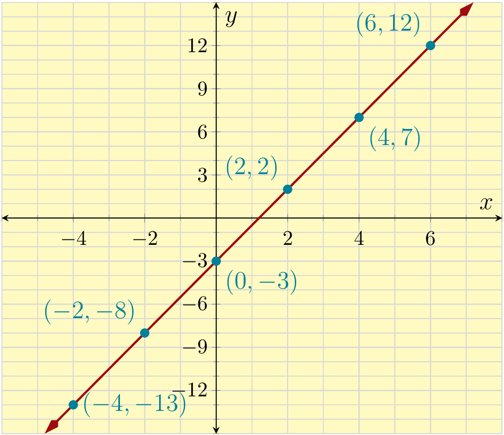
Make a graph of the linear equation \(y=\frac{5}{2}x-3\) by building a table of \(x\)- and \(y\)-values and plotting the points.
To create an easy-to-graph table of values, we should examine the formula and notice that if all of the \(x\)-values were multiples of \(2\text{,}\) then the fraction in the equation would cancel nicely and leave us with integer \(y\)-values.
| \(x\) | \(y=\frac{5}{2}x-3\) | Point |
| \(-4\) | \(\frac{5}{2}(\substitute{-4})-3\) \({}=-13\) |
\((-4,-13)\) |
| \(-2\) | \(\frac{5}{2}(\substitute{-2})-3\) \({}=-8\) |
\((-2,-8)\) |
| \(0\) | \(\frac{5}{2}(\substitute{0})-3\) \({}=-3\) |
\((0,-3)\) |
| \(2\) | \(\frac{5}{2}(\substitute{2})-3\) \({}=2\) |
\((2,2)\) |
| \(4\) | \(\frac{5}{2}(\substitute{4})-3\) \({}=7\) |
\((4,7)\) |
| \(6\) | \(\frac{5}{2}(\substitute{6})-3\) \({}=12\) |
\((6,12)\) |

Example 9.1.11.
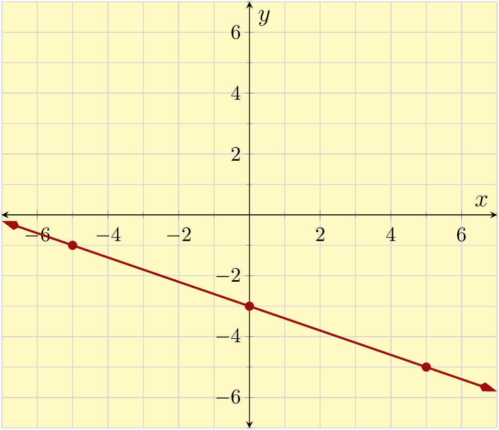
Create a table of ordered pairs and then make a plot of the equation \(y=-\frac{2}{5}x-3\text{.}\) Note that this equation is a linear equation, and we can see that the slope is negative. Therefore we should expect to see a downward sloping line as we view it from left to right. If we don't see that in the end, it suggests some mistake was made.
This time, with the slope having denominator \(5\text{,}\) it is wise to use multiples of \(5\) as the \(x\)-values.

Checkpoint 9.1.12.
Even when the equation is not a linear equation, this method (making a table of points) will work to help create a graph.
Example 9.1.13.
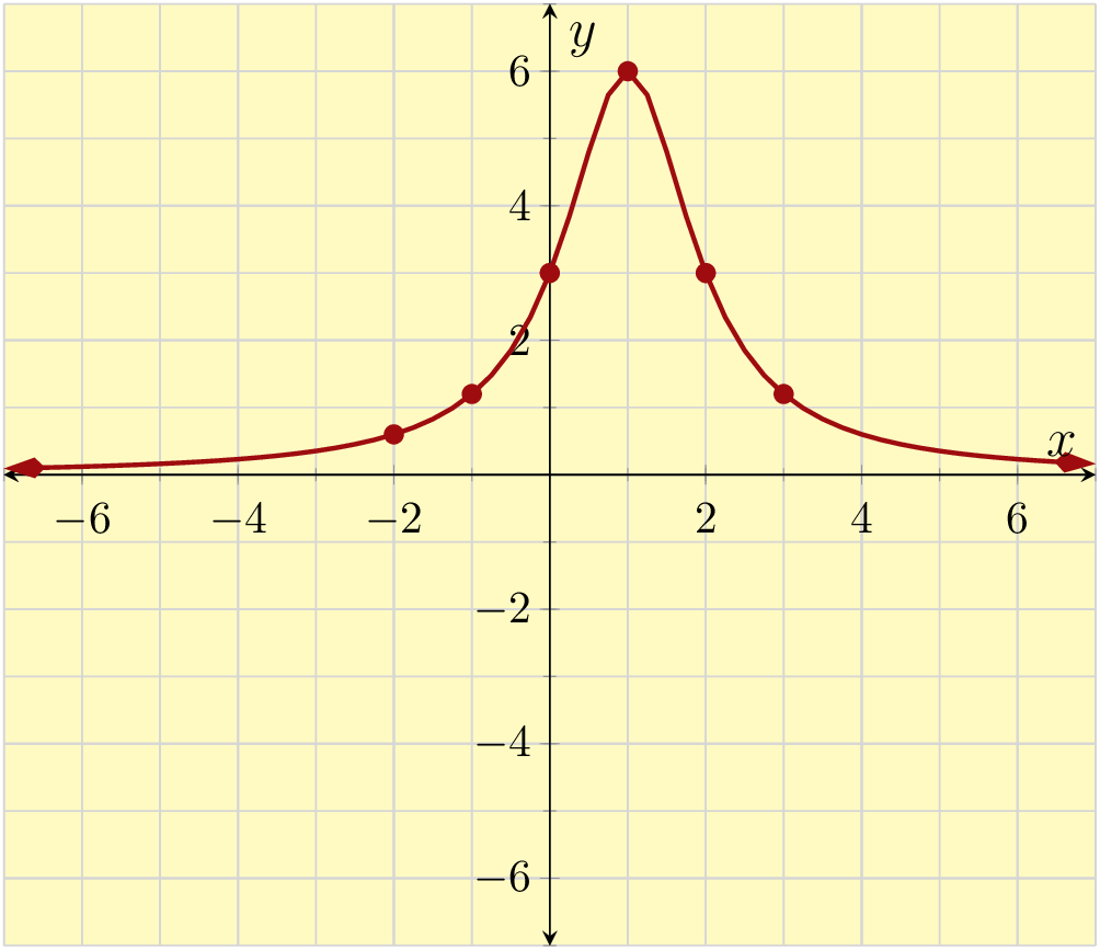
Create a table of ordered pairs and then make a plot of the equation \(y=\frac{6}{x^2-2x+2}\text{.}\)
The form of this equation is not one that we recognize yet. But the general approach for making a graph is still going to work out.
| \(x\) | \(y=\frac{6}{x^2-2x+2}\) | Point |
| \(-2\) | \(\frac{6}{(\substitute{-2})^2-2(\substitute{-2})+2}\) \({}=0.6\) |
\((-2,0.6)\) |
| \(-1\) | \(\frac{6}{(\substitute{-1})^2-2(\substitute{-1})+2}\) \({}=1.2\) |
\((-1,1.2)\) |
| \(0\) | \(\frac{6}{(\substitute{0})^2-2(\substitute{0})+2}\) \({}=3\) |
\((0,3)\) |
| \(1\) | \(\frac{6}{(\substitute{1})^2-2(\substitute{1})+2}\) \({}=6\) |
\((1,6)\) |
| \(2\) | \(\frac{6}{(\substitute{2})^2-2(\substitute{2})+2}\) \({}=3\) |
\((2,3)\) |
| \(3\) | \(\frac{6}{(\substitute{3})^2-2(\substitute{3})+2}\) \({}=1.2\) |
\((3,1.2)\) |

Subsection 9.1.3 Graphing Lines Using Intercepts
As noted earlier, sometimes the form of an equation suggests an alternative way that we could graph it. In the case of a linear equation, an alternative to making a table is to find the line's “intercepts”. These are the locations where the line crosses either the \(x\)-axis or the \(y\)-axis. In the case of a straight line, that is theoretically all you need to graph the complete line. Here, we review this approach. We also hope this example simply serves as a reminder of what intercepts are.
Recall that the standard form (3.7.1) of a line equation is \(Ax+By=C\) where where \(A\text{,}\) \(B\text{,}\) and \(C\) are three numbers (each of which might be \(0\text{,}\) although at least one of \(A\) and \(B\) must be nonzero). If a linear equation is given in standard form, we can relative easily find the line's \(x\)- and \(y\)-intercepts by substituting in \(y=0\) and \(x=0\text{,}\) respectively.
Example 9.1.14.
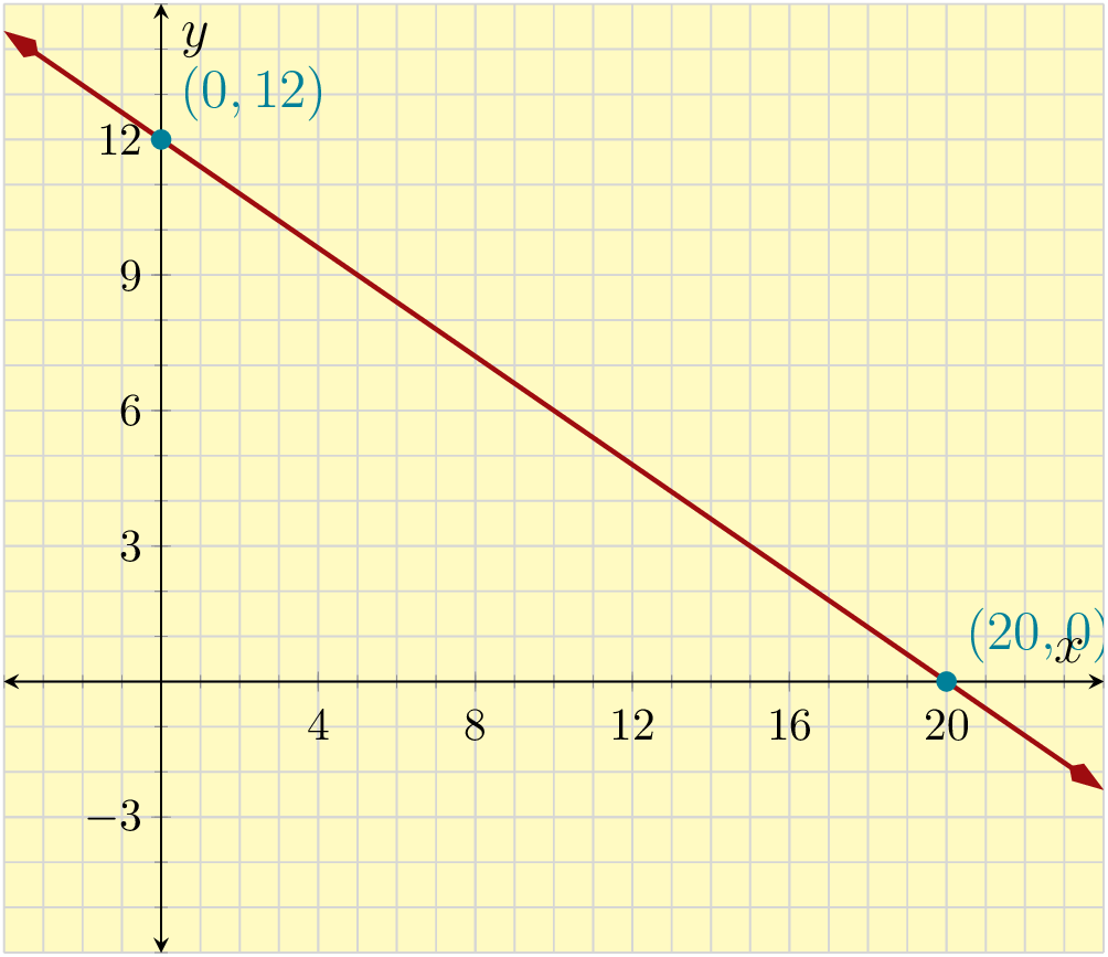
Find the intercepts of \(3x+5y=60\text{,}\) and then graph the equation given those intercepts.
To find the \(x\)-intercept, set \(y=0\) and solve for \(x\text{.}\)
So the \(x\)-intercept is the point \((\firsthighlight{20},\secondhighlight{0})\text{.}\)
To find the \(y\)-intercept, set \(x=0\) and solve for \(y\text{.}\)
So, the \(y\)-intercept is the point \((\firsthighlight{0},\secondhighlight{12})\text{.}\)

Checkpoint 9.1.16.
Exercises 9.1.4 Exercises
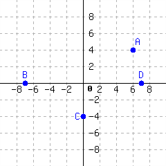
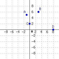
Identifying Coordinates
Plotting Points
3.
Sketch the points \((8,2)\text{,}\) \((5,5)\text{,}\) \((-3,0)\text{,}\) and \((2,-6)\) on a Cartesian plane.
4.
Sketch the points \((1,-4)\text{,}\) \((-3,5)\text{,}\) \((0,4)\text{,}\) and \((-2,-6)\) on a Cartesian plane.
Tables for Equations
5.
Make a table for the equation.
| \(x\) | \(y=4x\) |
6.
Make a table for the equation.
| \(x\) | \(y=8x\) |
7.
Make a table for the equation.
| \(x\) | \(y=6x+3\) |
8.
Make a table for the equation.
| \(x\) | \(y=8x-3\) |
9.
Make a table for the equation.
| \(x\) | \(y={\frac{10}{3}}x+10\) |
10.
Make a table for the equation.
| \(x\) | \(y={\frac{13}{10}}x - 8\) |
11.
Make a table for the equation.
| \(x\) | \(y=-{\frac{9}{8}}x - 6\) |
12.
Make a table for the equation.
| \(x\) | \(y={\frac{9}{8}}x - 4\) |
Graphs of Equations
13.
Create a table of ordered pairs and then make a plot of the equation \(y=2x+3\text{.}\)
14.
Create a table of ordered pairs and then make a plot of the equation \(y=-x-4\text{.}\)
15.
Create a table of ordered pairs and then make a plot of the equation \(y=\frac{4}{3}x\text{.}\)
16.
Create a table of ordered pairs and then make a plot of the equation \(y=-\frac{3}{4}x+2\text{.}\)
17.
Create a table of ordered pairs and then make a plot of the equation \(y=x^2+1\text{.}\)
18.
Create a table of ordered pairs and then make a plot of the equation \(y=(x-2)^2\text{.}\) Use \(x\)-values from \(0\) to \(4\text{.}\)
Lines and Intercepts
19.
Find the \(y\)-intercept and \(x\)-intercept of the line given by the equation. If a particular intercept does not exist, enter none into all the answer blanks for that row.
| \(x\)-value | \(y\)-value | Location (as an ordered pair) | |
| \(y\)-intercept | |||
| \(x\)-intercept |
20.
Find the \(y\)-intercept and \(x\)-intercept of the line given by the equation. If a particular intercept does not exist, enter none into all the answer blanks for that row.
| \(x\)-value | \(y\)-value | Location (as an ordered pair) | |
| \(y\)-intercept | |||
| \(x\)-intercept |
21.
Find the \(y\)-intercept and \(x\)-intercept of the line given by the equation. If a particular intercept does not exist, enter none into all the answer blanks for that row.
| \(x\)-value | \(y\)-value | Location (as an ordered pair) | |
| \(y\)-intercept | |||
| \(x\)-intercept |
22.
Find the \(y\)-intercept and \(x\)-intercept of the line given by the equation. If a particular intercept does not exist, enter none into all the answer blanks for that row.
| \(x\)-value | \(y\)-value | Location (as an ordered pair) | |
| \(y\)-intercept | |||
| \(x\)-intercept |
23.
Find the \(x\)- and \(y\)-intercepts of the line with equation \(5x-2y=10\text{.}\) Then find one other point on the line. Use your results to graph the line.
24.
Find the \(x\)- and \(y\)-intercepts of the line with equation \(5x-6y=-90\text{.}\) Then find one other point on the line. Use your results to graph the line.
25.
Find the \(x\)- and \(y\)-intercepts of the line with equation \(x+5y=-15\text{.}\) Then find one other point on the line. Use your results to graph the line.
26.
Find the \(x\)- and \(y\)-intercepts of the line with equation \(6x+y=-18\text{.}\) Then find one other point on the line. Use your results to graph the line.
27.
Make a graph of the line \(-5x-y=-3\text{.}\)
28.
Make a graph of the line \(x+5y=5\text{.}\)
29.
Make a graph of the line \(20x-4y=8\text{.}\)
30.
Make a graph of the line \(3x+5y=10\text{.}\)