In mathematics, we use functions to model real-life data. In this section, we will learn the definition of a function and related concepts.
Figure9.1.1 Alternative Video Lesson
Subsection9.1.1Introduction to Functions
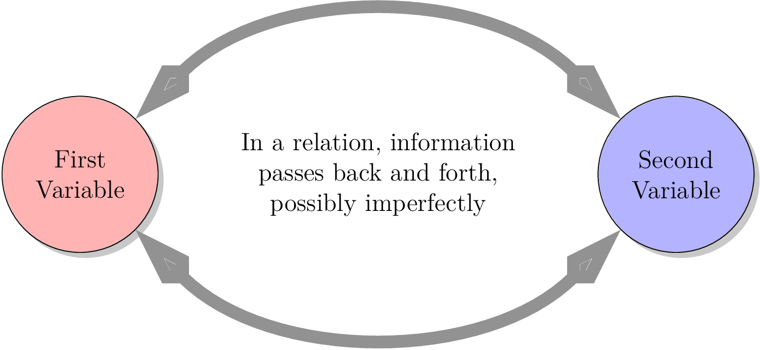
When working with two variables, we are interested in the relationship between those two variables. For example, consider the two variables of hare population and lynx population in a Canadian forest. If we know the value of one variable, are we able to determine the value of the second variable? If we know that one variable is increasing over time, do we know if the other is increasing or decreasing?
Figure9.1.2 In a relation, some knowledge of one variable implies some knowledge about the other
Definition9.1.3Relation
A relation is a very general situation between two variables, where having a little bit of information about one variable could tell you something about the other variable. For example, if you know the hare population is high this year, you can say the lynx population is probably increasing. So “hare population” and “lynx population” make a relation. If one of the variables is identified as the “first” variable, the relation's domain is the set of all values that variable can take. Likewise, the relation's range is the set of all values that the second variable can take.
We are not so much concerned with relations in this book. But we are interested in a special type of relation called a function. Informally, a function is a device that takes input values for one variable one by one, thinks about them, and gives respective output values one by one for the other variable.
Example9.1.4
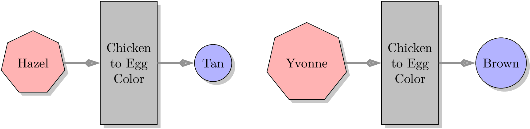
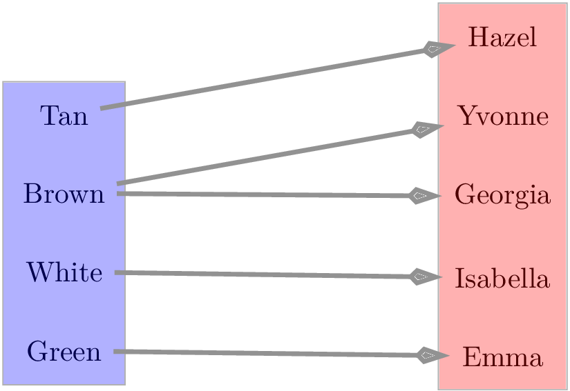
Mariana has \(5\) chickens: Hazel, Yvonne, Georgia, Isabella, and Emma. For the relation “Chicken to Egg Color,” the first variable (the input) is a chicken's name and the second variable (the output) is the color of that chicken's eggs. The relation's domain is the set of all of Mariana's chicken's names, and its range is the set of colors of her chicken's eggs. Figure 9.1.5 shows two inputs and their corresponding outputs.
Figure9.1.5 Two Pairs of Inputs and Outputs of the Relation “Chicken to Egg Color”
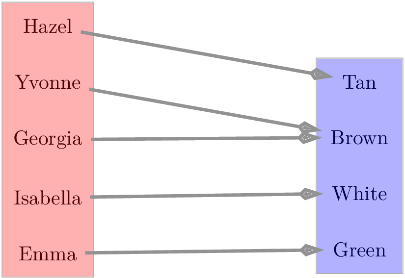
It would not be convenient to make diagrams like the ones in Figure 9.1.5 for all five chickens. There are too many inputs. Instead, Figure 9.1.6 represents the function graphically in a more concise way. The function's input variable is “chicken name,” and its output variable is “egg color.” Note that we are using the word “variable,” because the chicken names and egg colors vary depending on which individual chicken you choose.
where you read the ordered pair left to right, with the first value as an input and the second value as its output.
Definition9.1.7Function
In mathematics, a function is a relation between a set of inputs and a set of outputs with the property that each input is related to exactly one output.
In Figure 9.1.6, we can see each chicken's name (input) is related to exactly one output, so the relation “Chicken to Egg Color” qualifies as a function. Note that it is irrelevant that multiple inputs might related to the same output, like in \((\text{Yvonne}, \text{brown})\) and \((\text{Georgia}, \text{brown})\text{.}\) The point is that whichever chicken you are thinking about, you know exactly which color egg it lays.
Example9.1.8
Next, we will look at the “inverse” relation named “Egg Color to Chicken.” Here we consider the color of an egg to be the input, and want the output to be the name of a chicken. If the egg is green, we know it is Emma's. But what if the egg is brown?
In Figure 9.1.9, we can see the color brown (an input) is related to two outputs, Yvonne and Georgia. This disqualifies the relation “Egg Color to Chicken” from being a function. (It is still a relation, because in general knowing the egg color does give you some information about which chicken it may have come from.)
Functions are useful because they describe our ability to accurately predict a result. If we can predict something precisely every time, then there is a function involved.
Example9.1.10
If you go to the store and buy \(5\) two-dollar cans of soup, then you should predict that your total will be \(\$10\text{.}\) No matter if you buy the soup in the morning, afternoon, or evening. If it doesn't total \(\$10\text{,}\) then the cash register isn't functioning.
Example9.1.11
A vending machine is like a function. You push a button and the item you desired pops out. In this case, the inputs are all of the buttons that you can press, and the outputs are the kinds of candy bars, chip bags, etc. that can come out. The mechanics and electronics that connect the buttons with the items represent the function.
Going in a little further, if the button A1 delivers a bag of M&M's, then you would be surprised if you pressed A1 and got anything other than M&M's. In this case, the machine wouldn't be functioning and you would get upset at your prediction ability being taken away.
What if buttons A1 and B3 both delivered M&M's? Would that violate the definition a function?
No, the vending machine is still a function even if two buttons generate the same output. Remember that to be a function, each input must generate a single output; that output doesn't have to be unique for each input. So as long as each button generates the same item each time you press it, there can be two buttons that deliver the same item.
Example9.1.12
Some relations are not functions, because they can't be used to make \(100\%\) accurate predictions. For example, if you have a student's first name and want to determine their student ID number, you probably won't be able to look it up. For a common first name like “Michael,” there will be many student ID number possibilities. Multiple outputs for a single input make “student ID number” not be a function of “first name.”
On the other hand, if we exchange the variables and think of the ID number as the first variable, then there is only one student that ID number applies to, and there is only one official first name for that person. So “first name” is a function of “student ID number.”
Subsection9.1.3Algebraic Functions
Many functions have specific algebraic formulas to turn an input number into an output number. We explore some examples here.
Example9.1.13
Aylen is an electrician who is hired to install a new circuit. She charges \(\$111\) to come to your house and then, in addition, \(\$89\) per hour to do the work. If \(x\) represents the total number of hours that the job takes and \(y\) represents the total cost of her work, in dollars, then the equation \(y=89x+111\) relates the variables.
We know that at the end of the job, if Aylen worked \(x\) hours, you are going to have one bill that totals \(89x+111\text{.}\) This must mean that the bill is a function of the number of hours of labor. For every possible number of hours that she could work, you would only get one bill for that cost.
Context aside, the expression \(89x+111\) represents a function of \(x\text{,}\) because it can be used to turn an input number \(x\) into a specific output. In fact, every algebraic expression in one variable represents a function for similar reasons.
Example9.1.14
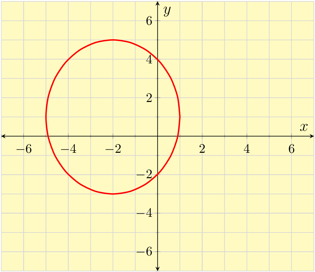
The equation \(x^2+y^2=25\) represents a relation that is not a function, where we view \(x\) as the “first variable” as usual. Remember that to not be a function, all we have to do is find one input that has two outputs. Let's pick a nice easy input number to test: \(x=4\text{.}\) Substituting this value gives us
At this point, we see that \(y\) could be \(3\) or \(y\) could be \(-3\text{.}\) There are two \(y\)-values for the single \(x\)-value, so that must mean that \(x^2+y^2=25\) cannot represent a function.
Checkpoint9.1.15
Subsection9.1.4Function Notation
We know that the equation \(y=5x+3\) represents \(y\) as a function of \(x\text{,}\) because for each \(x\)-value (input), there is only one \(y\)-value (output). If we want to determine the value of the output when the input is \(2\text{,}\) we'd replace \(x\) with \(2\) and find the value of \(y\text{:}\)
Our end result is that \(y=13\text{.}\) Well, \(y\) is \(13\text{,}\) but only in the situation when \(x\) is \(2\text{.}\) In general, for other inputs, \(y\) is not going to be \(13\text{.}\) So the equation \(y=13\) is lacking in the sense that it is not communicating everything we might want to say. It does not communicate the value of \(x\) that we used. Function notation will allow us to communicate both the input and the output at the same time. It will also allow us to give each function a name, which is helpful when we have multiple functions.
Functions can have names just like variables. The most common function name is \(f\text{,}\) since “f” stands for “function.” A letter like \(f\) doesn't stand for a single number though. Instead, it represents an input-output relation like we've been discussing in this section.
We will write equations like \(y=f(x)\text{,}\) and what we mean is:
“y equals f of x”
the function's name is \(f\)
the input variable is \(x\)
the parentheses following the \(f\) surround the input; they do not indicate multiplication
the output variable is \(y\)
Remark9.1.16
Parentheses have a lot of uses in mathematics. Their use with functions is very specific, and it's important to note that \(f\) is not being multiplied by anything when we write \(f(x)\text{.}\) With function notation, the parentheses specifically are just meant to indicate the input by surrounding the input.
Example9.1.17
The expression \(f(x)\) is read as “\(f\) of \(x\text{,}\)” and the expression \(f(2)\) is read as “\(f\) of \(2\text{.}\)” Be sure to practice saying this correctly while reading.
The expression \(f(2)\) means that \(2\) is being treated as an input, and the function \(f\) is turning it into an output. And then \(f(2)\) represents that actual output number.
Remark9.1.18
The most common letters used to represent functions are \(f,g,\) and \(h\text{.}\) The most common variables we use are \(x\text{,}\) \(y\text{,}\) and \(z\text{.}\) But we can use any function name and any input and output variable. When dealing with functions in context, it often makes sense to use meaningful function names and variables. For example, if we are modeling temperature of a cup of coffee as a function of time with a function \(C\text{,}\) we could use \(T=C(t)\text{,}\) where \(T\) is the temperature (in degrees Fahrenheit) after \(t\) minutes.
Subsection9.1.5Evaluating Functions
When we determine a function's value for a specific input, this is known as evaluating a function. To do so, we replace the input with the numerical value given and determine the associated output.
When using function notation, instead of writing \(5x+3\) or \(y=5x+3\text{,}\) we often write something like \(f(x)=5x+3\text{.}\) We are saying that the rule for function \(f\) is to use the expression \(5x+3\text{.}\) To find \(f(2)\text{,}\) wherever you see \(x\) in the formula \(f(x)=5x+3\text{,}\) substitute in \(2\text{:}\)
Our end result is that \(f(2)=13\text{,}\) which tells us that \(f\) turns \(2\) into \(13\text{.}\) In other words, when the input is \(2\text{,}\) the output will be \(13\text{.}\)
Checkpoint9.1.19Functions with Algebraic Formulas
A function may be described by explicitly listing many inputs and their corresponding outputs in a table.
Example9.1.20Functions given in Table Form
Temperature readings for Portland, OR, on a given day are recorded in Table 9.1.21 . Let \(f(x)\) be the temperature in degrees Fahrenheit \(x\) hours after midnight.
\(x\text{,}\) hours after midnight
\(0\)
\(1\)
\(2\)
\(3\)
\(4\)
\(5\)
\(6\)
\(7\)
\(8\)
\(9\)
\(10\)
\(f(x)\text{,}\) temperature in °F
\(45\)
\(44\)
\(42\)
\(42\)
\(43\)
\(44\)
\(45\)
\(48\)
\(49\)
\(50\)
\(53\)
Table9.1.21 Recorded Temperatures in Portland, OR, on a certain day
What was the temperature at midnight?
Find \(f(9)\text{.}\) Explain what this function value represents in the context of the problem.
To determine the temperature at midnight, we look in the table where \(x=0\) and see that the output is \(45\text{.}\) Using function notation, we would write:
In context, this means that at 9AM the temperature was 50 °F.
A function may be described using a graph, where the horizontal axis corresponds to possible input values (the domain), and the vertical axis corresponds to possible output values (the range).
Example9.1.22Functions in Graphical Form
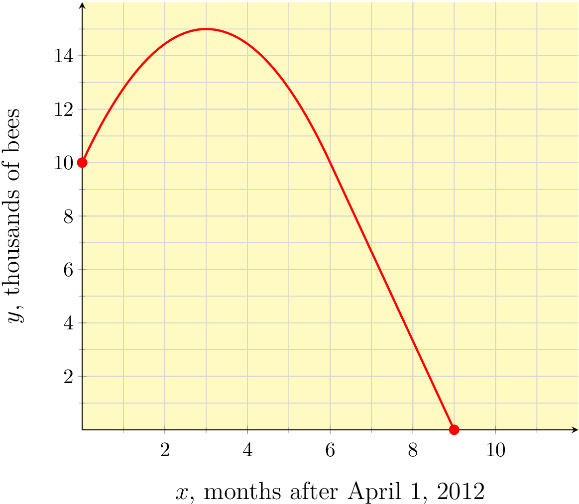
A colony of bees settled in Zahid's backyard in 2012. Let \(B(x)\) be the number of bees in the colony (in thousands) \(x\) months after April 1, 2012. A graph of \(y=B(x)\) is shown in Figure 9.1.23.
Determine the number of bees in the colony on July 1, 2012.
Find \(B(0)\text{.}\) Explain what this function value represents in the context of the problem.
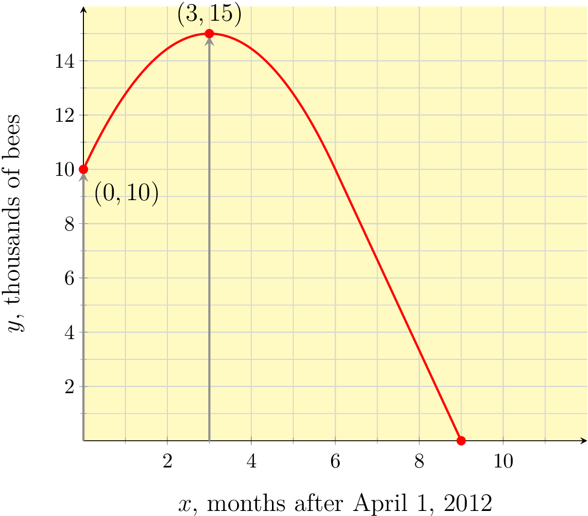
Since July 1 is \(3\) months after April 1, that means we need to use \(x=3\) as the input. On the horizontal axis, find \(3\text{,}\) as in Figure 9.1.24. Looking straight up or down, we find the point \((3,15)\) on the curve. That means that \(B(3)=15\text{.}\) A value of \(y=15\) when \(x=3\) tells us that there were \(15{,}000\) bees \(3\) months after April 1, 2012 (on July 1, 2012).
To find \(B(0)\text{,}\) we recognize that this will be the output of the function when \(x=0\text{.}\) The point \((0,10)\) on the graph of \(y=B(x)\) tells us that \(B(0)=10\text{.}\) In the context of this problem, this means on April 1, 2012 there were \(10{,}000\) bees in the colony.
Subsection9.1.6Solving Equations That Have Function Notation
Evaluating a function and solving an equation that has function notation in it are two separate things. Students understandably mix up these two tasks, because they are two sides of the same coin. Evaluating a function means that you know an input (typically, an \(x\)-value) and then you calculate an output (typically, a \(y\)-value). Solving an equation that has function notation in it is the opposite process. You know an output (typically, a \(y\)-value) and then you determine all the inputs that could have led to that output (typically, \(x\)-values).
Checkpoint9.1.25Functions with Algebraic Formulas
In Checkpoint 9.1.19, we found the function value when given the input, which we refer to as evaluating a function. To solve an equation that has function notation in it, we need to solve for the value of the variable that makes an equation true, just like in any other equation.
Example9.1.26Functions given in Table Form
In Example 9.1.20, we evaluated a function given in table form, using Table 9.1.21. Let's use that function to solve equations.
Solve \(f(x)=48\text{.}\) Explain what this solution set represents in context.
To solve \(f(x)=48\text{,}\) we need to find the value of \(x\) that makes the equation true. Looking at the table, we look at the outputs and see that the output \(48\) occurs when \(x=7\text{.}\) In abstract terms, the solution set is \(\{7\}\text{.}\) In context, this means that the temperature was 48 °F at 7AM.
To determine when the temperature was 44 °F, we look in the table to see where the output was 44 °F. This occurs when \(x=1\) and again when \(x=5\text{.}\) In abstract terms, the solution set is \(\{1,5\}\text{.}\) In context, this means that the temperature was 44 °F at 1AM and again at 5AM.
Example9.1.27Functions given in Graphical Form
In Example 9.1.22, we evaluated a function given in graphical form, using Figure 9.1.23. Now let's use that function to solve some equations.
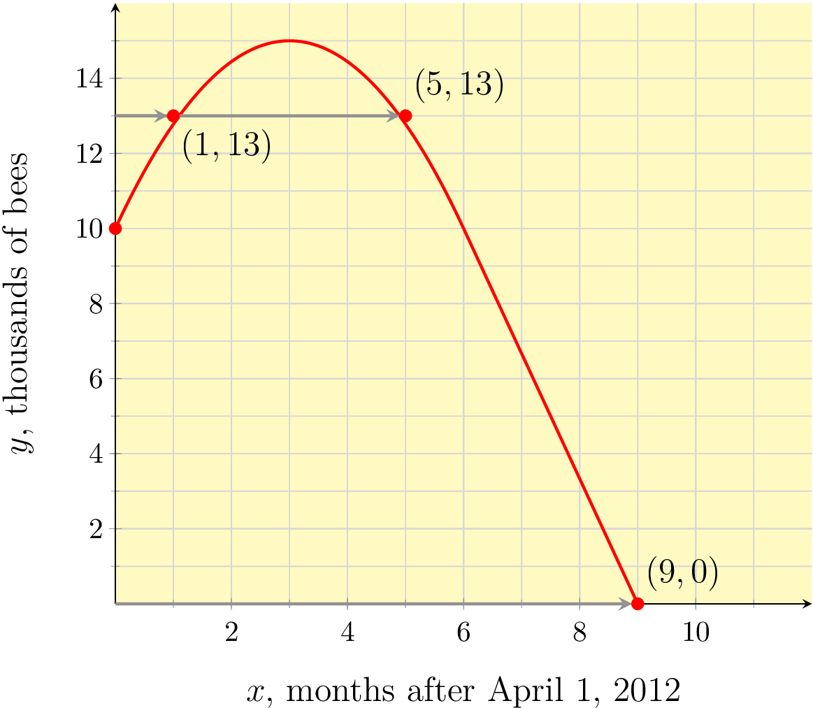
Solve \(B(x)=0\text{.}\) Explain what the solution set represents in the context of the problem.
To solve \(B(x)=0\text{,}\) we need to consider that number \(0\) as an output value, so it belongs on the vertical axis in Figure 9.1.28. Moving straight right or left, we find the point \((9,0)\) is on the graph, and that tells us that \(B(x)=0\) when \(x=9\text{.}\) Abstractly, the solution set is \(\{9\}\text{.}\) In the context of this problem, this means there were \(0\) bees in the colony \(9\) months after April 1, 2012 (on January 1, 2013).
To determine when the number of bees reached \(13{,}000\text{,}\) we need to recognize that \(13\) is an output value and locate it on the vertical axis. Moving straight right or left, we find (approximately) that the points \((1,13)\) and \((5,13)\) are on the graph. This means \(x\approx 1\) and \(x\approx 5\) are solutions. Abstractly, the solution set is approximately \(\{1, 5\}\text{.}\) In context, there will be \(13,000\) bees in the colony approximately 1 month after April 1, 2012 (on May 1, 2012) and again 5 months after April 1, 2012 (on September 1, 2012).
Earlier we defined the domain and range of a relation. We repeat those definitions more formally here, specifically for functions.
Definition9.1.29Domain and Range
Given a function \(f\text{,}\) the domain of \(f\) is the collection of all valid input values for \(f\text{.}\) The range of \(f\) is the collection of all possible output values of \(f\text{.}\)
When working with functions, a common necessary task is to determine the function's domain and range. Also, the ability to identify domain and range is strong evidence that a person really understands the concepts of domain and range.
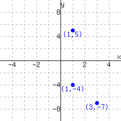
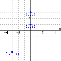
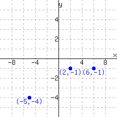
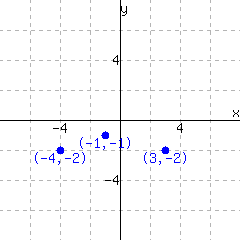
Example9.1.30Functions Defined by Ordered Pairs
The function \(f\) is defined by the ordered pairs
The ordered pairs tell us that \(f(1)=2\text{,}\) \(f(3)=-2\text{,}\) etc. So the valid input values are \(1\text{,}\) \(3\text{,}\) \(5\text{,}\) \(7\text{,}\) and \(9\text{.}\) This means the domain is the set \(\{1,3,5,7,9\}\text{.}\)
Similarly, the ordered pairs tell us that \(2\text{,}\) \(-2\text{,}\) \(-4\text{,}\) and \(6\) are possible output values. Notice that the output \(2\) happened twice, but it only needs to be listed in this collection once. The range of \(f\) is \(\{2,-2,-4,6\}\text{.}\)
Example9.1.31Functions in Table Form
For each function defined using a table, state the domain and range.
The table tells us that \(g(-2)=5\text{,}\) \(g(-1)=5\text{,}\) etc. So the valid input values are \(-2\text{,}\) \(-1\text{,}\) \(0\text{,}\) \(1\text{,}\) and \(2\text{.}\) This means the domain of \(g\) is the set \(\{-2,-1,0,1,2\}\text{.}\)
The only output evident from this table is \(5\text{,}\) so the range of \(g\) is the set \(\{5\}\text{.}\)
The table tells us that \(h(0)=8\text{,}\) \(h(1)=6\text{,}\) etc. So the valid input values are \(0\text{,}\) \(1\text{,}\) \(2\text{,}\) \(3\text{,}\) and \(4\text{.}\) This means the domain of \(h\) is the set \(\{0,1,2,3,4\}\text{.}\)
Similarly, the table shows us that the possible outputs are \(8\text{,}\) \(6\text{,}\) \(4\text{,}\) \(2\text{,}\) and \(0\text{.}\) So the range of \(h\) is the set \(\{8,6,4,2,0\}\text{.}\)
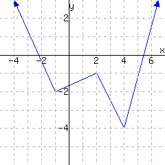
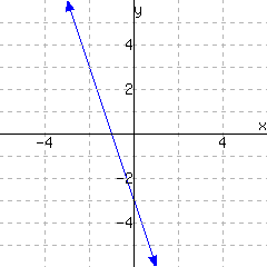
Example9.1.32Functions in Graphical Form
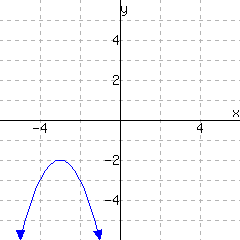
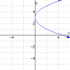
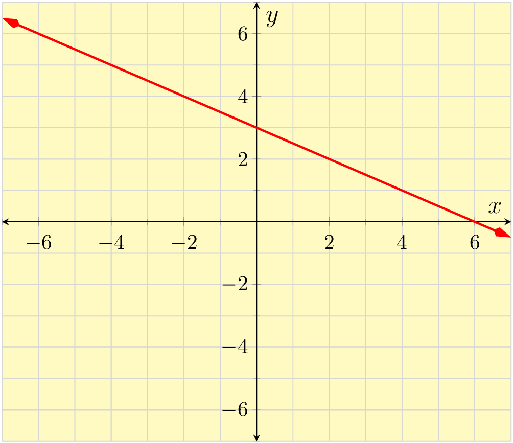
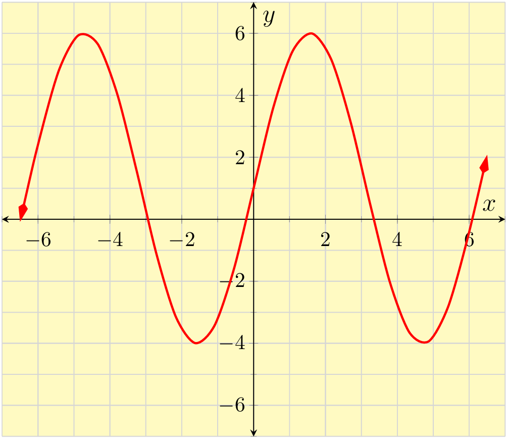
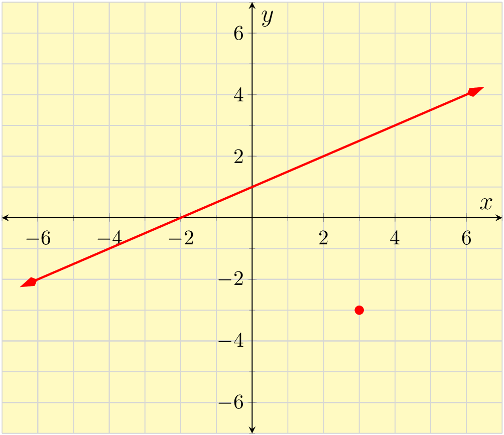
Functions are graphed in Figure 9.1.33 through Figure 9.1.35. For each one, find its domain and range. In previous examples the domain and range were finite sets and we used set notation braces to communicate them. In these examples, the domain and range will be intervals, and so we use interval notation.
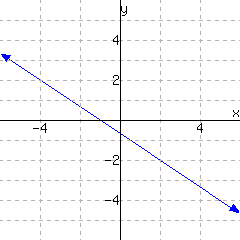
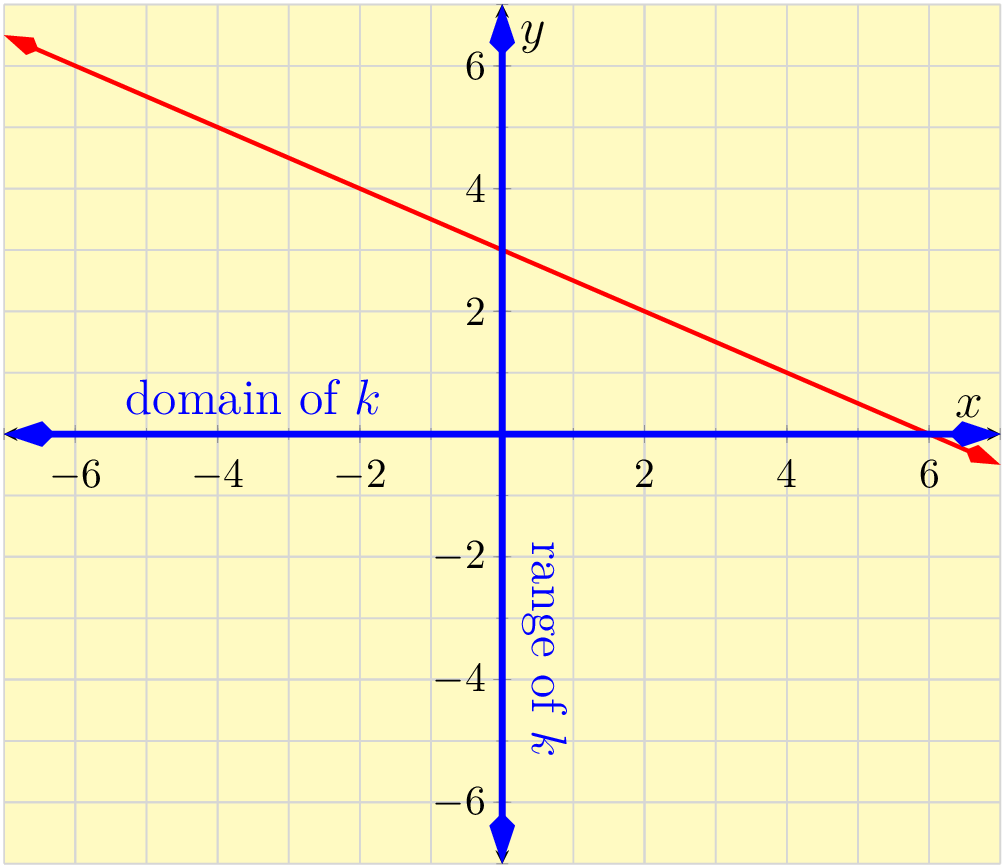
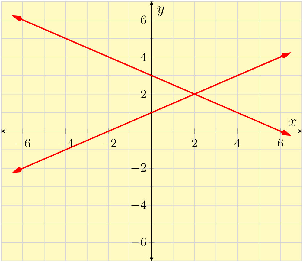
To find the domain of \(k\text{,}\) we look left and right across the \(x\)-axis. No matter where we look on the \(x\)-axis, we can look straight up or down and find a point on the graph. So no matter what input we imagine, there is always an corresponding output. Therefore the domain is all real numbers, which we write as \((-\infty,\infty)\text{.}\)
Similarly, to find the range of \(k\text{,}\) we look up and down over the entire \(y\)-axis. No matter where we stop on the \(y\)-axis, we will be able to move straight left or right and find a point on the graph. So no matter what output we imagine, there is always an input that leads to that output. Therefore the range is also \((-\infty,\infty)\text{.}\)
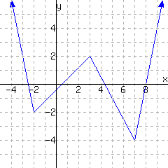
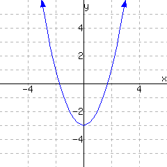
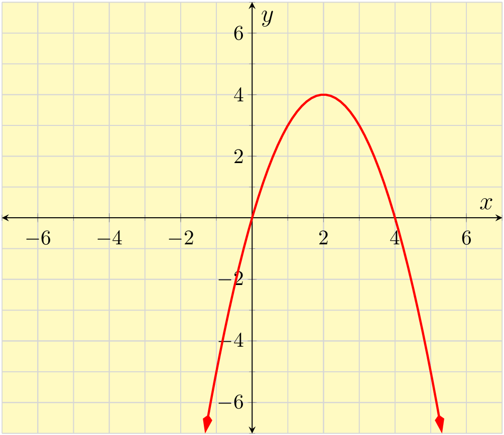
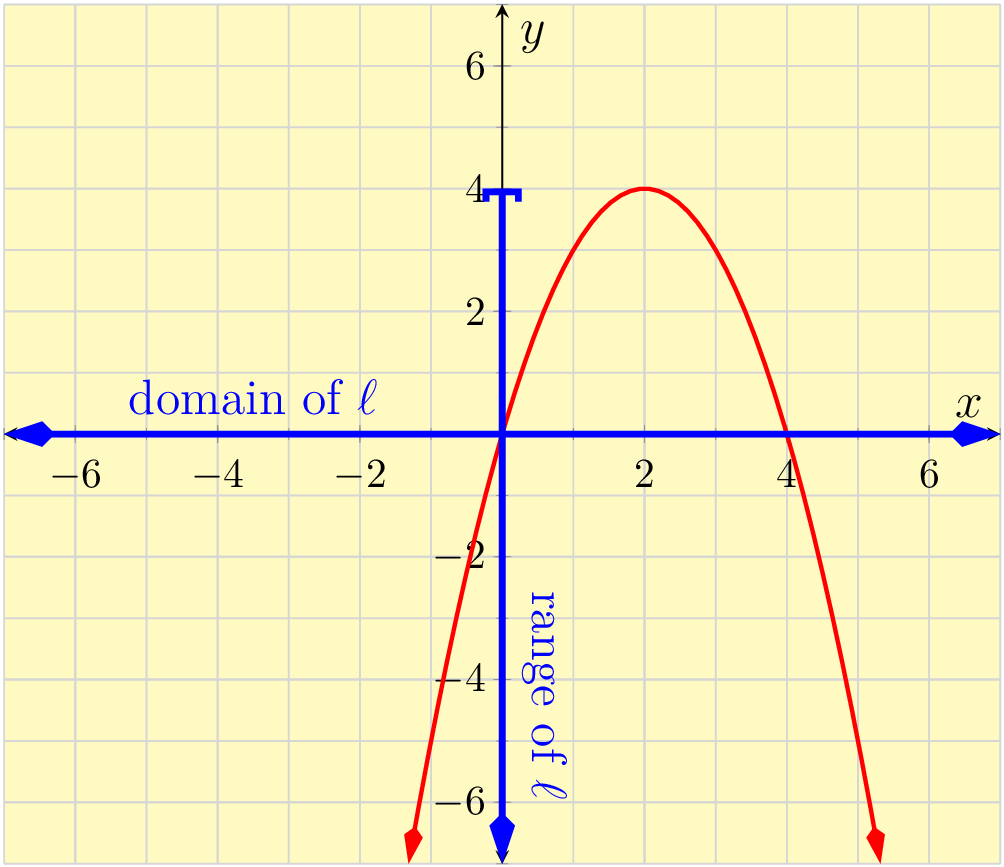
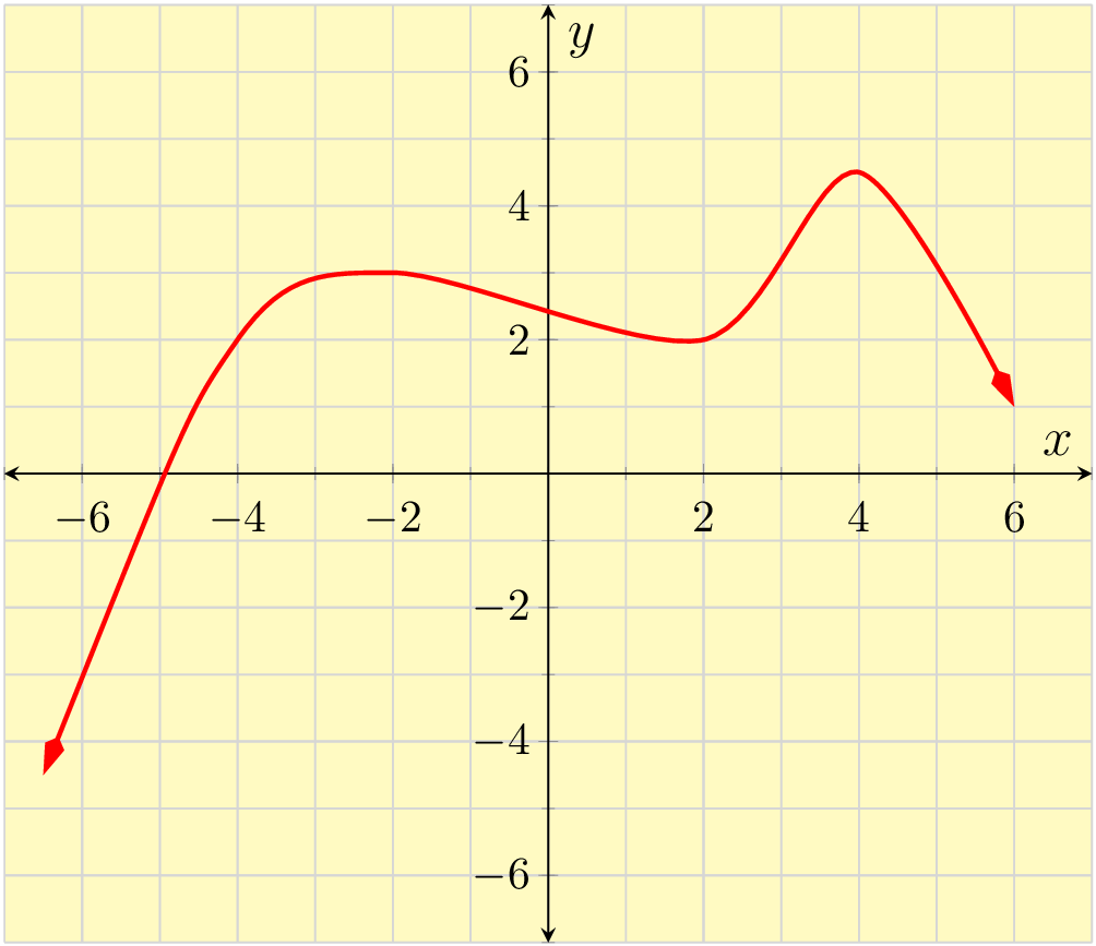
To find the domain of \(\ell\text{,}\) we look left and right across the entire \(x\)-axis. No matter where we stop on the \(x\)-axis, we will be able to move straight up or down and find a point on the graph. (Although if we are far out left or right, we will have to look very far down to find that point.) So no matter what input we imagine, there is always an output to this function. Therefore the domain is \((-\infty,\infty)\text{.}\)
To find the range of \(\ell\text{,}\) we look up and down over the entire \(y\)-axis. For \(y\)-values larger than \(4\text{,}\) if we look straight left or right, there is no point on the curve. Only with \(y\)-values \(4\) and under can we find an input that leads to such an output. So the range is all real numbers less than or equal to \(4\text{.}\) In interval notation, that is \((-\infty,4]\text{.}\)
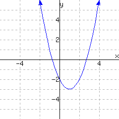
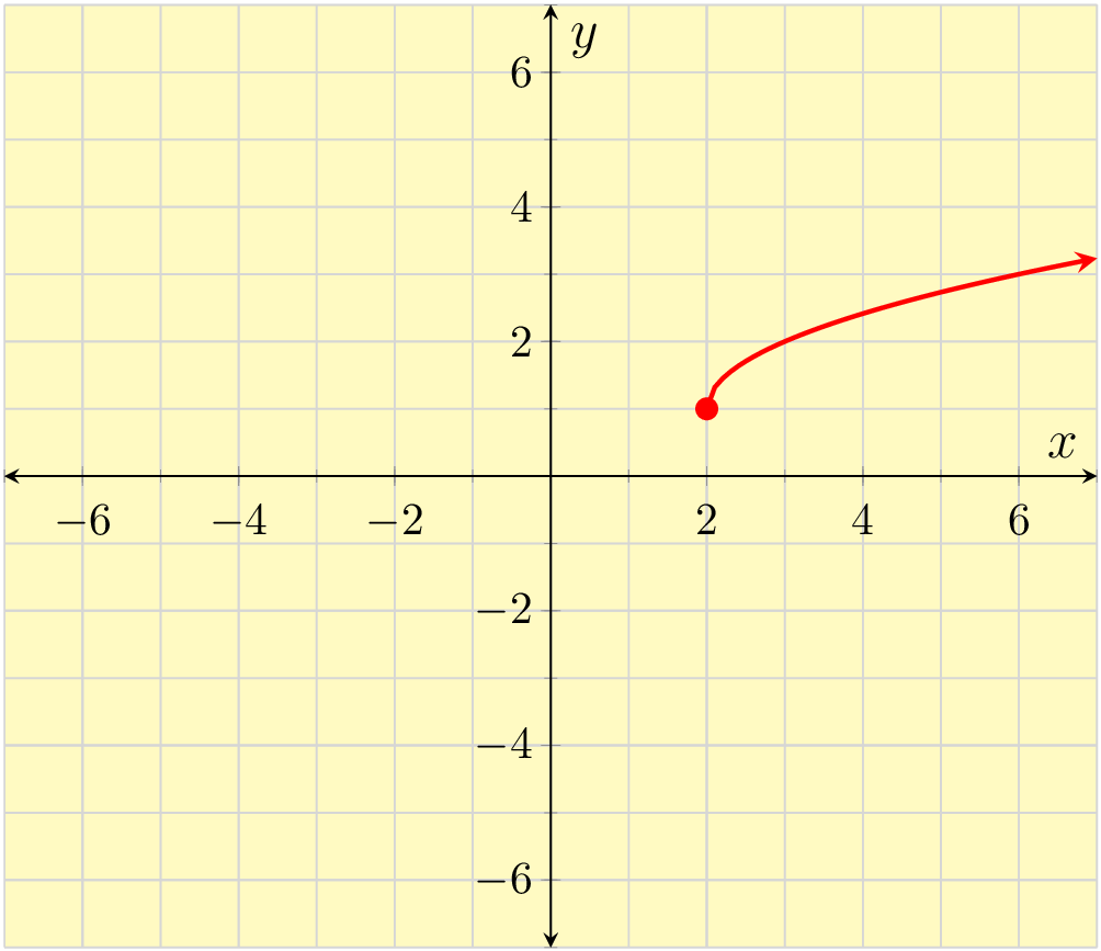
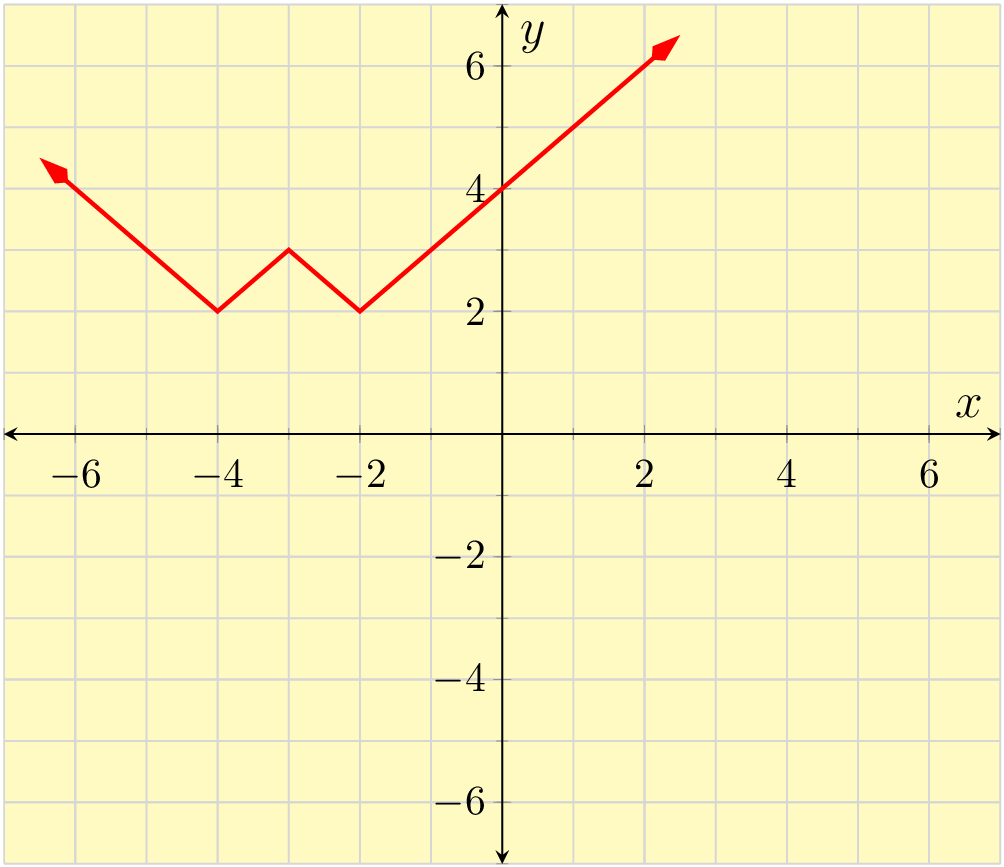
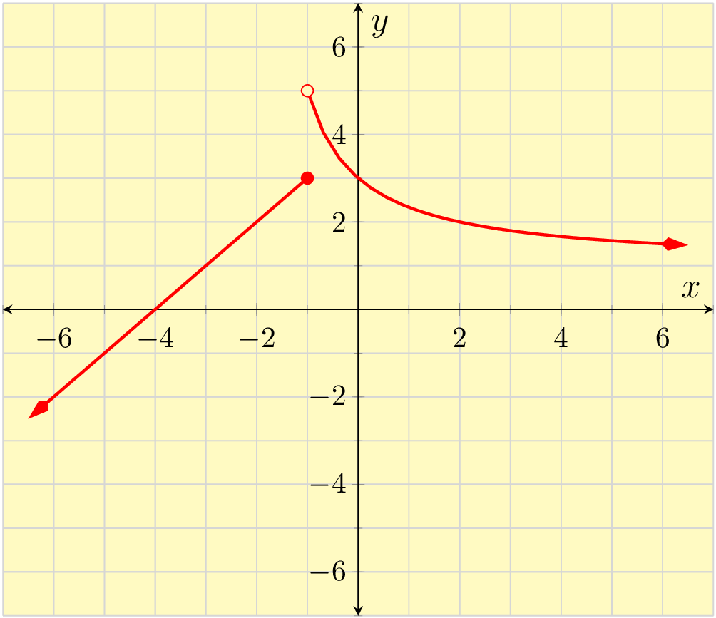
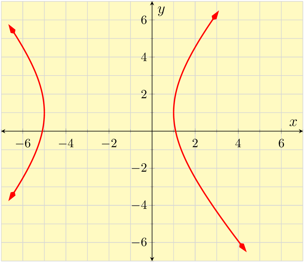
To find the domain of \(m\text{,}\) we look left and right across the entire \(x\)-axis. For an \(x\)-value less than \(2\text{,}\) there is no point on the curve directly above or below that \(x\)-value. So the graph is not telling you what \(m(x)\) would be. Only for \(x\)-values \(2\) and greater do we get an output value. So the domain is \([2,\infty)\text{.}\)
To find the range of \(m\text{,}\) we look up and down over the entire \(y\)-axis. For \(y\)-values less than \(1\text{,}\) if we look straight left or right, there is no point on the curve. Only with \(y\)-values \(1\) and greater can we find an input that leads to such an output. So the range is all real numbers greater than or equal to \(1\text{.}\) In interval notation, that is \([1,\infty)\text{.}\)
Subsection9.1.8Determining if a Relation is a Function
We have seen functions that are defined using a verbal description, using an equation, using a list of ordered pairs, using a table, and using a graph. With all of these things, you might have a relation that is not actually a function. (We have seen a few examples of these as well.) Determining whether or not a given relation actually defines a function is another task that demonstrates actual understanding of the concept of a function.
Example9.1.39Verbally Described Relations
In the introduction, we discussed the relation between the variables of hare population and lynx population. These variables are related—for one thing, if the hare population is high, you will have information about the lynx population: it will probably be increasing because there is plenty of food.
But is this relation a function? Suppose that one year you know the hare population is \(100{,}000\) and the lynx population is \(2000\text{.}\) Isn't it possible that some other year, the hare population is \(100{,}000\) again, but the lynx population is something different like \(3000\text{?}\) Knowing one value of the first variable does not guarantee exactly one value of the second variable. So this relation is not a function.
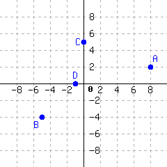
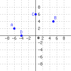
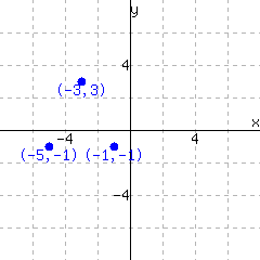
Checkpoint9.1.40Sets of Ordered Pairs
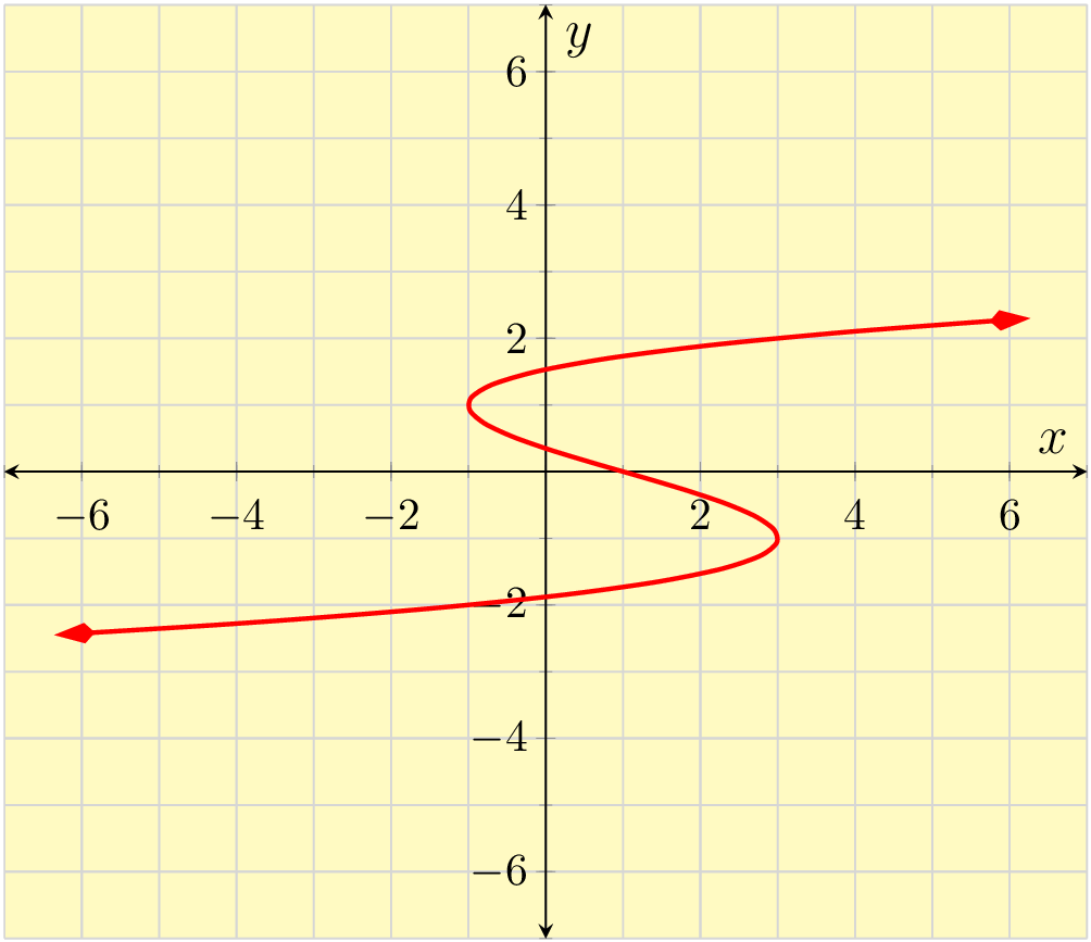
To determine if a relation that is represented graphically is a function, we need to visually determine if each input corresponds to exactly one output. How could that not happen? Somewhere on the horizontal axis, there would be a number, and looking straight up or straight down from there, you would find at least two points on the graph.
This thinking gives rise to the vertical line test.
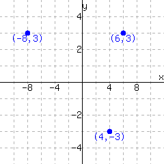
Fact9.1.41Vertical Line Test
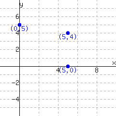
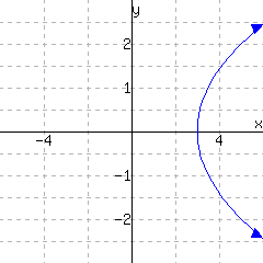
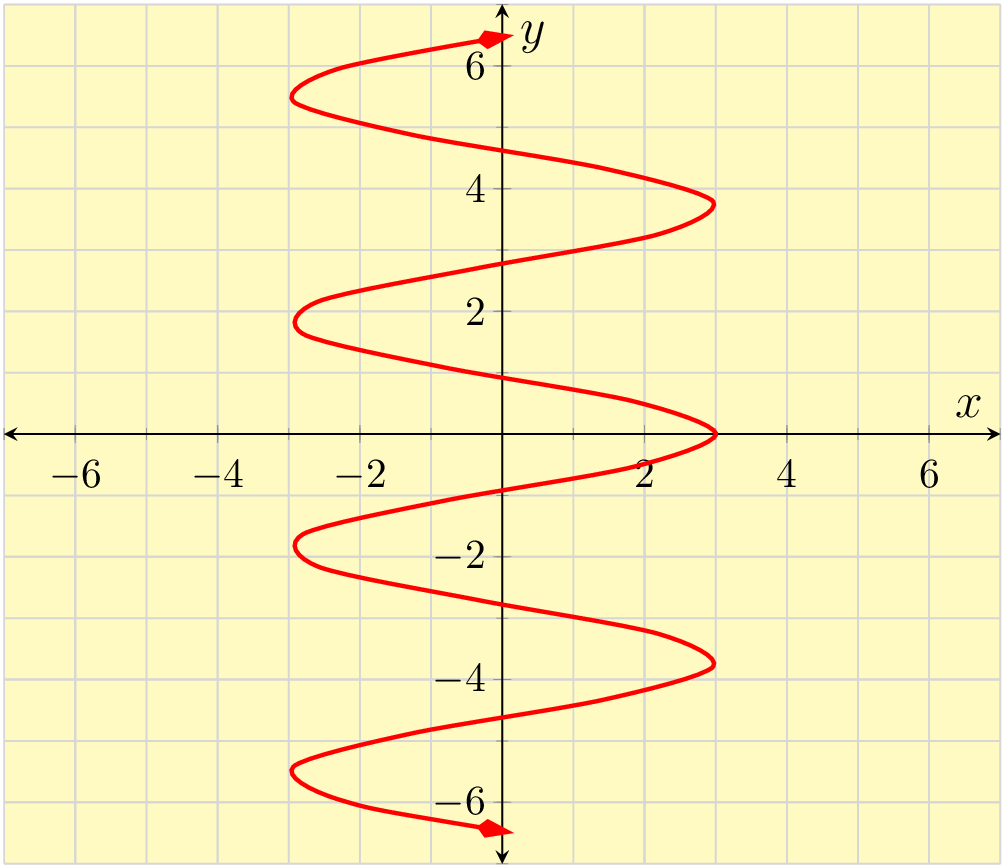
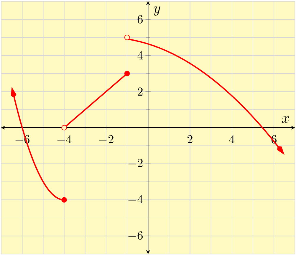
If any vertical line passes through the graph of a relation more than once, then \(y\) is not a function of \(x\) in the graph.
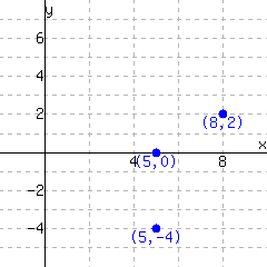
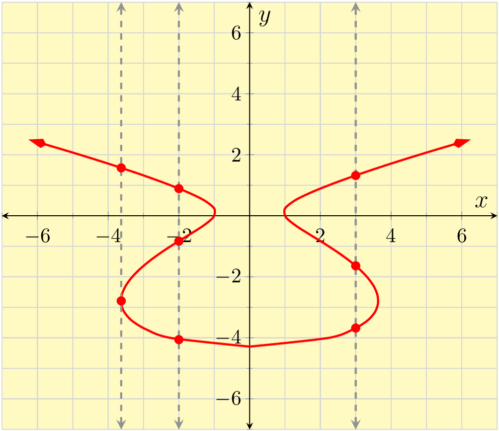
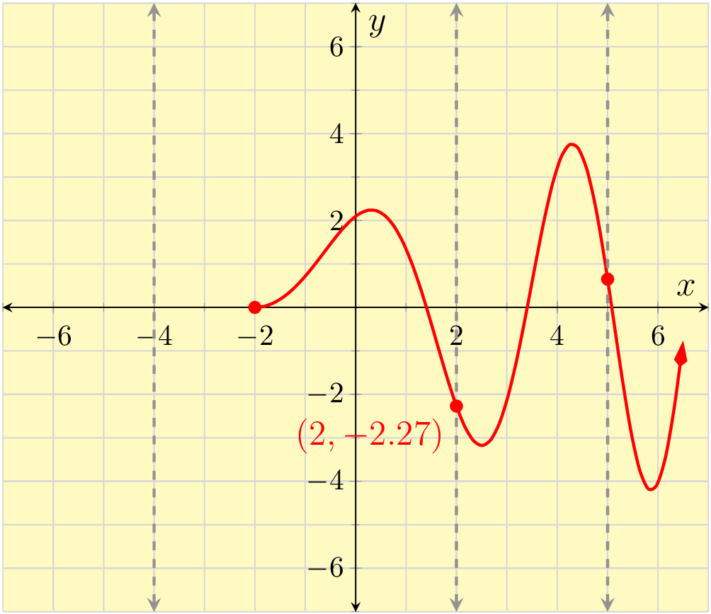
Figure9.1.43 Fails the Vertical Line TestFigure9.1.44 Passes the Vertical Line Test
In Figure 9.1.43, we can see that there are vertical lines that pass through the graph more than once. This means that this graph does not represent a function. The issue is that supposing it were a function \(f\text{,}\) then what would \(f(3)\) be? The graph suggests it could be three different things: \(\approx1.3\text{,}\) \(\approx-1.6\text{,}\) and \(\approx-3.7\text{.}\) With no clear single output for the input \(3\text{,}\) we don't have a function.
However, in Figure 9.1.44, we see that all vertical lines pass through the graph one time (or not at all). Therefore, this graph does represent a function. If we name the function \(g\text{,}\) the domain of \(g\) is only numbers greater than or equal to \(2\text{.}\) And for such numbers, the graphs shows us exactly one output for each input. For example, the graph shows us that \(g(2)\approx-2.27\text{.}\)
For relations in table form, we can determine if it makes a function by again checking to see if multiple outputs are ever associated with a single input.
Example9.1.45Functions in Table Form
For each relation shown in Table 9.1.46 through Table 9.1.48, determine if \(y\) is a function of \(x\text{.}\)
This relation represents a function as each input corresponds to exactly one output. For instance, the input \(-2\) only corresponds to the output \(5\) and no other output. (Note that it does not matter that multiple inputs correspond to the same output \(5\text{.}\))
\(x\)
\(-2\)
\(-1\)
\(0\)
\(1\)
\(2\)
\(y\)
\(5\)
\(5\)
\(5\)
\(5\)
\(5\)
Table9.1.46 A function?
This relation represents a function as each input corresponds to exactly one output. For instance, the input \(0\) only corresponds to the output \(8\) and no other output.
\(x\)
\(0\)
\(1\)
\(2\)
\(3\)
\(4\)
\(y\)
\(8\)
\(6\)
\(4\)
\(2\)
\(0\)
Table9.1.47
This relation does not represent a function as some of the inputs correspond to more than one output. In particular, the input of \(2\) corresponds to both \(7\) and \(9\) for outputs.
If \(H(1)=0\text{,}\) then the point is on the graph of \(H\text{.}\)
If \({\left(1,6\right)}\) is on the graph of \(H\text{,}\) then \(H(1)=\).
58
If \(K(8)=12\text{,}\) then the point is on the graph of \(K\text{.}\)
If \({\left(8,13\right)}\) is on the graph of \(K\text{,}\) then \(K(8)=\).
59
If \(f(y)=t\text{,}\) then the point is on the graph of \(f\text{.}\)
The answer is not a specific numerical point, but one with variables for coordinates.
60
If \(f(x)=r\text{,}\) then the point is on the graph of \(f\text{.}\)
The answer is not a specific numerical point, but one with variables for coordinates.
61
If \({\left(r,x\right)}\) is on the graph of \(g\text{,}\) then \(g(r)=\).
62
If \({\left(y,r\right)}\) is on the graph of \(h\text{,}\) then \(h(y)=\).
Function Notation in Context
63
Suppose that \(M\) is the function that computes how many miles are in \(x\) feet. Find the algebraic rule for \(M\text{.}\) (If you do not know how many feet are in one mile, you can look it up on Google.)
\(M(x)=\)
Evaluate \(M(19000)\) and interpret the result:
There are about miles in feet.
64
Suppose that \(K\) is the function that computes how many kilograms are in \(x\) pounds. Find the algebraic rule for \(K\text{.}\) (If you do not know how many pounds are in one kilogram, you can look it up on Google.)
\(K(x)=\)
Evaluate \(K(214)\) and interpret the result.
Something that weighs pounds would weigh about kilograms.
65
Stephanie started saving in a piggy bank on her birthday. The function \(f(x)={3x+2}\) models the amount of money, in dollars, in Stephanie’s piggy bank. The independent variable represents the number of days passed since her birthday.
Interpret the meaning of \(f(4)=14\text{.}\)
A. Four days after Stephanie started her piggy bank, there were \(\$14\) in it.
B. Fourteen days after Stephanie started her piggy bank, there were \(\$4\) in it.
C. The piggy bank started with \(\$14\) in it, and Stephanie saves \(\$4\) each day.
D. The piggy bank started with \(\$4\) in it, and Stephanie saves \(\$14\) each day.
66
Sherial started saving in a piggy bank on her birthday. The function \(f(x)={5x+3}\) models the amount of money, in dollars, in Sherial’s piggy bank. The independent variable represents the number of days passed since her birthday.
Interpret the meaning of \(f(1)=8\text{.}\)
A. The piggy bank started with \(\$1\) in it, and Sherial saves \(\$8\) each day.
B. The piggy bank started with \(\$8\) in it, and Sherial saves \(\$1\) each day.
C. One days after Sherial started her piggy bank, there were \(\$8\) in it.
D. Eight days after Sherial started her piggy bank, there were \(\$1\) in it.
67
An arcade sells multi-day passes. The function \(g(x)={{\frac{1}{4}}x}\) models the number of days a pass will work, where \(x\) is the amount of money paid, in dollars.
Interpret the meaning of \(g(12)={3}\text{.}\)
A. If a pass costs \(\$12\text{,}\) it will work for \(3\) days.
B. Each pass costs \(\$12\text{,}\) and it works for \(3\) days.
C. If a pass costs \(\$3\text{,}\) it will work for \(12\) days.
D. Each pass costs \(\$3\text{,}\) and it works for \(12\) days.
68
An arcade sells multi-day passes. The function \(g(x)={{\frac{1}{2}}x}\) models the number of days a pass will work, where \(x\) is the amount of money paid, in dollars.
Interpret the meaning of \(g(4)={2}\text{.}\)
A. Each pass costs \(\$2\text{,}\) and it works for \(4\) days.
B. Each pass costs \(\$4\text{,}\) and it works for \(2\) days.
C. If a pass costs \(\$4\text{,}\) it will work for \(2\) days.
D. If a pass costs \(\$2\text{,}\) it will work for \(4\) days.
69
Bobbi will spend \({\$105}\) to purchase some bowls and some plates. Each bowl costs \({\$2}\text{,}\) and each plate costs \({\$3}\text{.}\) The function \(p(b)={-{\frac{2}{3}}b+35}\) models the number of plates Bobbi will purchase, where \(b\) represents the number of bowls Bobbi will purchase.
Interpret the meaning of \(p(39)={9}\text{.}\)
A. \(\$9\) will be used to purchase bowls, and \(\$39\) will be used to purchase plates.
B. If \(9\) bowls are purchased, then \(39\) plates will be purchased.
C. If \(39\) bowls are purchased, then \(9\) plates will be purchased.
D. \(\$39\) will be used to purchase bowls, and \(\$9\) will be used to purchase plates.
70
Lisa will spend \({\$135}\) to purchase some bowls and some plates. Each bowl costs \({\$2}\text{,}\) and each plate costs \({\$3}\text{.}\) The function \(p(b)={-{\frac{2}{3}}b+45}\) models the number of plates Lisa will purchase, where \(b\) represents the number of bowls Lisa will purchase.
Interpret the meaning of \(p(30)={25}\text{.}\)
A. \(\$25\) will be used to purchase bowls, and \(\$30\) will be used to purchase plates.
B. If \(25\) bowls are purchased, then \(30\) plates will be purchased.
C. If \(30\) bowls are purchased, then \(25\) plates will be purchased.
D. \(\$30\) will be used to purchase bowls, and \(\$25\) will be used to purchase plates.
71
Barbara will spend \({\$125}\) to purchase some bowls and some plates. Each plate costs \({\$3}\text{,}\) and each bowl costs \({\$5}\text{.}\) The function \(q(x)={-{\frac{3}{5}}x+25}\) models the number of bowls Barbara will purchase, where \(x\) represents the number of plates to be purchased.
Interpret the meaning of \(q(5)={22}\text{.}\)
A. \(5\) plates and \(22\) bowls can be purchased.
B. \(22\) plates and \(5\) bowls can be purchased.
C. \(\$22\) will be used to purchase bowls, and \(\$5\) will be used to purchase plates.
D. \(\$5\) will be used to purchase bowls, and \(\$22\) will be used to purchase plates.
72
Sharell will spend \({\$360}\) to purchase some bowls and some plates. Each plate costs \({\$9}\text{,}\) and each bowl costs \({\$8}\text{.}\) The function \(q(x)={-{\frac{9}{8}}x+45}\) models the number of bowls Sharell will purchase, where \(x\) represents the number of plates to be purchased.
Interpret the meaning of \(q(24)={18}\text{.}\)
A. \(\$18\) will be used to purchase bowls, and \(\$24\) will be used to purchase plates.
B. \(18\) plates and \(24\) bowls can be purchased.
C. \(24\) plates and \(18\) bowls can be purchased.
D. \(\$24\) will be used to purchase bowls, and \(\$18\) will be used to purchase plates.
73
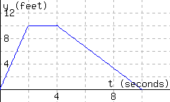
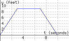
The following figure has the graph \(y=d(t)\text{,}\) which models a particle’s distance from the starting line in feet, where \(t\) stands for time in seconds since timing started.
A. The particle was \(3.33333\) feet away from the starting line \(8\) seconds since timing started.
B. In the first \(3.33333\) seconds, the particle moved a total of \(8\) feet.
C. The particle was \(8\) feet away from the starting line \(3.33333\) seconds since timing started.
D. In the first \(8\) seconds, the particle moved a total of \(3.33333\) feet.
Solve \(d(t)={5}\) for \(t\text{.}\) \(t=\)
Interpret the meaning of part c’s solution(s):
A. The article was \(5\) feet from the starting line \(7\) seconds since timing started.
B. The article was \(5\) feet from the starting line \(1\) seconds since timing started, and again \(7\) seconds since timing started.
C. The article was \(5\) feet from the starting line \(1\) seconds since timing started, or \(7\) seconds since timing started.
D. The article was \(5\) feet from the starting line \(1\) seconds since timing started.
74
The following figure has the graph \(y=d(t)\text{,}\) which models a particle’s distance from the starting line in feet, where \(t\) stands for time in seconds since timing started.


![the previous graph of function l with a thick line along the x-axis; this indicates that the domain is all real numbers; there is an interval on the y-axis with a bracket opening down at 4 and an arrow pointing downward; this indicates that the range is (-infinity, 4]](images/image-1010.svg)


