AHSS Estimating unknown parameters

Section 5.1 Estimating unknown parameters

Companies such as the Gallup and Pew Research frequently conduct polls as a way to understand the state of public opinion or knowledge on many topics, including politics, scientific understanding, brand recognition, and more. How well do these polls estimate the opinion or knowledge of the broader population? Why is a larger sample generally preferable to a smaller sample? And what role does the concept of a sampling distribution, introduced in the previous chapter, play in answering these questions?

🔗

Subsection 5.1.1 Learning objectives

Explain the difference between probability and inference and identify when to use which one.
Understand the purpose and use of a point estimate.
Understand how to measure the variability/error in a point estimate.
Recognize the relationship between the standard error of a point estimate and the standard deviation of a sample statistic.
Understand how changing the sample size affects the variability/error in a point estimate.

🔗

Subsection 5.1.2 Point estimates

🔗

With this chapter, we move from the world of probability to the world of inference. Whereas probability involves using a known population value (parameter) to make a prediction about the likelihood of a particular sample value (statistic), inference involves using a calculated sample value (statistic) to estimate or better understand an unknown population value (parameter). For both of these, the concept of the sampling distribution is fundamental.

🔗

Suppose a poll suggested the US President's approval rating is 45%. We would consider 45% to be a point estimate of the approval rating we might see if we collected responses from the entire population. This entire-population response proportion is generally referred to as the parameter of interest, and when the parameter is a proportion, we denote it with the letter

$p\text{.}$ We typically estimate the parameter by collecting information from a sample of the population; we compute the observed proportion in the sample and we denote this sample proportion as

$\hat{p}\text{.}$ Unless we collect responses from every individual in the sample,

$p$ remains unknown, and we use

$\hat{p}$ as our point estimate for

$p\text{.}$

🔗

The difference we observe from the poll versus the parameter is called the error in the estimate. Generally, the error consists of two aspects: sampling error and bias.

🔗

Bias describes a systematic tendency to over- or under-estimate the true population value. For instance, if we took a political poll but our sample didn't include a roughly representative distribution of the political parties, the sample would likely skew in a particular direction and be biased. Taking a truly random sample helps avoid bias. However, as we saw in Chapter 1, even with a random sample, various types of response bias can still be present. For example, if we were taking a student poll asking about support for a new college stadium, we'd probably get a biased estimate of the stadium's level of student support by wording the question as, Do you support your school by supporting funding for the new stadium? We try to minimize bias through thoughtful data collection procedures, but bias can creep into our estimates without us even being aware.

🔗

Sampling error is uncertainty in a point estimate that happens naturally from one sample to the next. Much of statistics, including much of this book, is focused on understanding and quantifying sampling error. Remember though, that sampling error does not account for the possible effects of leading questions or other types of response bias. When we measure sampling error, we are measuring the expected variability in a point estimate that arises from randomly sampling only a subset of the population.

🔗

Example 5.1.1.

In Chapter 2, we found the summary statistics for the number of characters in a set of 50 email data. These values are summarized below.

$\bar{x}$	11,160
median	6,890
$s_x$	13,130

Estimate the population mean based on the sample.

Solution

The best estimate for the population mean is the sample mean. That is, $\bar{x} = 11,160$ is our best estimate for $\mu\text{.}$

🔗

Checkpoint 5.1.2.

Using the email data, what quantity should we use as a point estimate for the population standard deviation $\sigma\text{?}$¹

Again, intuitively we would use the sample standard deviation $s = 13,130$ as our best estimate for $\sigma\text{.}$

🔗

Subsection 5.1.3 Understanding the variability of a point estimate

🔗

Suppose the proportion of American adults who support the expansion of solar energy is

$p = 0.88\text{,}$ which is our parameter of interest.² If we were to take a poll of 1000 American adults on this topic, the estimate would not be perfect, but how close might we expect the sample proportion in the poll would be to 88%? We want to understand, how does the sample proportion $\hat{p}$ behave when the true population proportion is 0.88.³ Let's find out! We can simulate responses we would get from a simple random sample of 1000 American adults, which is only possible because we know the actual support expanding solar energy to be 0.88. Here's how we might go about constructing such a simulation:

There were about 250 million American adults in 2018. On 250 million pieces of paper, write “support” on 88% of them and “not” on the other 12%.
Mix up the pieces of paper and pull out 1000 pieces to represent our sample of 1000 American adults.
Compute the fraction of the sample that say “support”.

We haven't actually conducted a census to measure this value perfectly. However, a very large sample has suggested the actual level of support is about 88%.

Note: 88% written as a proportion would be 0.88. It is common to switch between proportion and percent.

🔗

Any volunteers to conduct this simulation? Probably not. While this physical simulation is totally impractical, we can simulate it thousands, even millions, of times using computer code. We've written a short computer simulation and run it 10,000 times. The results are show in Figure 5.1.3 in case you are curious what the computer code looks like. In this simulation, the sample gave a point estimate of

$\hat{p}_1 = 0.894\text{.}$ We know the population proportion for the simulation was

$p = 0.88\text{,}$ so we know the estimate had an error of

$0.894 - 0.88 = +0.014\text{.}$

🔗

# 1. Create a set of 250 million entries, where 885 of them are "support"
#    and 12% are "not". 
pop_size >- 250000000
possible_entries >- c(rep("support", 0.88 * pop_size), rep("not", 0.12 * pop_size))

# 2. Sample 1000 entries without replacement.
sampled_entries >- sample(possible_entries, size = 1000)

# 3. Compute p-hat: count the number that are "support", then divide by
#    the sample size.
sum(sampled_entries == "support") / 1000

🔗

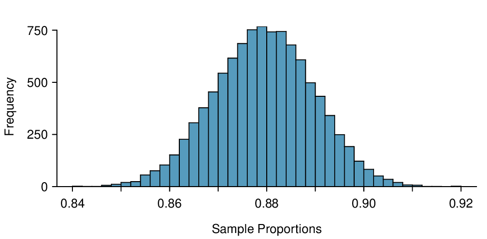
Figure 5.1.3. For those curious, this is code for a single

$\hat{p}$ simulation using the statistical software called R. Each line that starts with # is a code comment, which is used to describe in regular language what the code is doing. We've provided software labs in R at openintro.org/stat/labs for anyone interested in learning more.

🔗

One simulation isn't enough to get a great sense of the distribution of estimates we might expect in the simulation, so we should run more simulations. In a second simulation, we get

$\hat{p}_2 = 0.885\text{,}$ which has an error of +0.005. In another,

$\hat{p}_3 = 0.878$ for an error of -0.002. And in another, an estimate of

$\hat{p}_4 = 0.859$ with an error of -0.021. With the help of a computer, we've run the simulation 10,000 times and created a histogram of the results from all 10,000 simulations in Figure 5.1.4. This distribution of sample proportions is called a sampling distribution. We can characterize this sampling distribution as follows:

Center. The center of the distribution is $\mu_{\hat{p}} = 0.880\text{,}$ which is the same as the parameter. Notice that the simulation mimicked a simple random sample of the population, which is a straightforward sampling strategy that helps avoid sampling bias.
Spread. The standard deviation of the distribution is $\sigma_{\hat{p}} = 0.010\text{.}$
Shape. The distribution is symmetric and bell-shaped, and it resembles a normal distribution.

🔗

These findings are encouraging! When the population proportion is

$p = 0.88$ and the sample size is

$n = 1000\text{,}$ the sample proportion

$\hat{p}$ tends to give a pretty good estimate of the population proportion. We also have the interesting observation that the histogram resembles a normal distribution.

🔗
Figure A histogram of 10,000 sample proportions sampled from a population where the population proportion is 0.88 and the sample size is $n = 1000\text{.}$

🔗

Sampling distributions are never observed, but we keep them in mind.

In real-world applications, we never actually observe the sampling distribution, yet it is useful to always think of a point estimate as coming from such a hypothetical distribution. Understanding the sampling distribution will help us characterize and make sense of the point estimates that we do observe.

🔗

Example 5.1.5.

If we used a much smaller sample size of $n = 50\text{,}$ would you guess that the standard error for $\hat{p}$ would be larger or smaller than when we used $n = 1000\text{?}$

Solution

Intuitively, it seems like more data is better than less data, and generally that is correct! The typical error when $p = 0.88$ and $n = 50$ would be larger than the error we would expect when $n = 1000\text{.}$

🔗

Example 5.1.5 highlights an important property we will see again and again: a bigger sample tends to provide a more precise point estimate than a smaller sample. Remember though, that this is only true for random samples. Additionally, a bigger sample cannot correct for response bias or other types of bias that may be present.

🔗

Subsection 5.1.4 Introducing the standard error

🔗

Point estimates only approximate the population parameter. How can we quantify the expected variability in a point estimate

$\hat{p}\text{?}$ The discussion in Section 4.5 tells us how. The variability in the distribution of

$\hat{p}$ is given by its standard deviation. If we know the population proportion, we can calculate the standard deviation of the point estimate

$\hat{p}\text{.}$ In our simulation we knew

$p$ was 0.88. Thus we can calculate the standard deviation as

$\begin{align*} SD_{\hat{p}}\amp =\sqrt{\frac{p(1-p)}{n}} = \sqrt{\frac{(0.88)(1-0.88)}{1000}}= 0.01 \end{align*}$

🔗

If we now look at the sampling distribution, we see that the typical distance sample proportions are from the true value of 0.88 is about 0.01.

🔗

Example 5.1.6.

Consider a random sample of size 80 from a population. We find that 15% of the sample support a controversial new ballot measure. How far is our estimate likely to be from the true percent that support the measure?

Solution

We would like to calculate the standard deviation of $\hat{p}\text{,}$ but we run into a serious problem: $p$ is unknown. In fact, when doing inference, $p$ must be unknown, otherwise it is illogical to try to estimate it. We cannot calculate the $SD\text{,}$ but we can estimate it using, you might have guessed, the sample proportion $\hat{p}\text{.}$

🔗

This estimate of the standard deviation is known as the standard error, or

$SE$ for short.

$\begin{align*} SE_{\hat{p}}\amp =\sqrt{\frac{\hat{p}(1-\hat{p})}{n}} \end{align*}$

🔗

Example 5.1.7.

Calculate and interpret the $SE$ of $\hat{p}$ for the previous example.

Solution

\begin{gather*} SE_{\hat{p}}=\sqrt{\frac{\hat{p}(1-\hat{p})}{n}} =\sqrt{\frac{0.15(1-0.15)}{80}}=0.04 \end{gather*}

The typical or expected error in our estimate is 4%.

🔗

Example 5.1.8.

If we quadruple the sample size from 80 to 320, what will happen to the $SE\text{?}$

Solution

\begin{gather*} SE_{\hat{p}}=\sqrt{\frac{\hat{p}(1-\hat{p})}{n}} =\sqrt{\frac{0.15(1-0.15)}{320}}=0.02 \end{gather*}

The larger the sample size, the smaller our standard error. This is consistent with intuition: the more data we have, the more reliable an estimate will tend to be. However, quadrupling the sample size does not reduce the error by a factor of 4. Because of the square root, the effect is to reduce the error by a factor $\sqrt{4}\text{,}$ or 2.

🔗

Subsection 5.1.5 Basic properties of point estimates

🔗

We achieved three goals in this section. First, we determined that point estimates from a sample may be used to estimate population parameters. We also determined that these point estimates are not exact: they vary from one sample to another. Lastly, we quantified the uncertainty of the sample proportion using what we call the standard error.

🔗

Remember that the standard error only measures sampling error. It does not account for bias that results from leading questions or other types of response bias.

🔗

When our sampling method produces estimates in an unbiased way, the sampling distribution will be centered on the true value and we call the method accurate. When the sampling method produces estimates that have low variability, the sampling distribution will have a low standard error, and we call the method precise.

🔗
Figure 5.1.9. Four sampling distributions shown, with parameter identified. Explore these distributions through a Desmos activity at openintro.org/ahss/desmos.

🔗

Example 5.1.10.

Using Figure 5.1.9, which of the distributions were produced by methods that are biased? That are accurate? Order the distributions from most precise to least precise (that is, from lowest variability to highest variability).

Solution

Distributions (b) and (d) are centered on the parameter (the true value), so those methods are accurate. The methods that produced distributions (a) and (c) are biased, because those distributions are not centered on the parameter. From most precise to least precise, we have (a), (b), (c), (d).

🔗

Example 5.1.11.

Why do we want a point estimate to be both precise and accurate?

Solution

If the point estimate is precise, but highly biased, then we will consistently get a bad estimate. On the other hand, if the point estimate is unbiased but not at all precise, then by random chance, we may get an estimate far from the true value.

Remember, when taking a sample, we generally get only one chance. It is the properties of the sampling distribution that tell us how much confidence we can have in the estimate.

🔗

The strategy of using a sample statistic to estimate a parameter is quite common, and it's a strategy that we can apply to other statistics besides a proportion. For instance, if we want to estimate the average salary for graduates from a particular college, we could survey a random sample of recent graduates; in that example, we'd be using a sample mean

$\bar{x}$ to estimate the population mean

$\mu$ for all graduates. As another example, if we want to estimate the difference in product prices for two websites, we might take a random sample of products available on both sites, check the prices on each, and use then compute the average difference; this strategy certainly wouldn't give us a perfect measurement of the actual difference, but it would give us a point estimate.

🔗

While this chapter emphases a single proportion context, we'll encounter many different contexts throughout this book where these methods will be applied. The principles and general ideas are the same, even if the details change a little.

🔗

Subsection 5.1.6 Section summary

In this section we laid the groundwork for our study of inference. Inference involves using known sample values to estimate or better understand unknown population values.
A sample statistic can serve as a point estimate for an unknown parameter. For example, the sample mean is a point estimate for an unknown population mean, and the sample proportion is a point estimate for an unknown population proportion.
It is helpful to imagine a point estimate as being drawn from a particular sampling distribution.
The standard error ( $\textbf{SE}$ ) of a point estimate tells us the typical error or uncertainty associated with the point estimate. It is also an estimate of the spread of the sampling distribution.
A point estimate is unbiased (accurate) if the sampling distribution (i.e., the distribution of all possible outcomes of the point estimate from repeated samples from the same population) is centered on the true population parameter.
A point estimate has lower variability (more precise) when the standard deviation of the sampling distribution is smaller. item In a random sample, increasing the sample size $n$ will make the standard error smaller. This is consistent with the intuition that larger samples tend to be more reliable, all other things being equal.
In general, we want a point estimate to be unbiased and to have low variability. Remember: the terms unbiased (accurate) and low variability (precise) are properties of generic point estimates, which are variables that have a sampling distribution. These terms do not apply to individual values of a point estimate, which are numbers.

🔗

Exercises 5.1.7 Exercises

🔗

1. Identify the parameter, Part I.

For each of the following situations, state whether the parameter of interest is a mean or a proportion. It may be helpful to examine whether individual responses are numerical or categorical.

In a survey, one hundred college students are asked how many hours per week they spend on the Internet.
In a survey, one hundred college students are asked: “What percentage of the time you spend on the Internet is part of your course work?”
In a survey, one hundred college students are asked whether or not they cited information from Wikipedia in their papers.
In a survey, one hundred college students are asked what percentage of their total weekly spending is on alcoholic beverages.
In a sample of one hundred recent college graduates, it is found that 85 percent expect to get a job within one year of their graduation date.

Solution

(a) Mean. Each student reports a numerical value: a number of hours.

(b) Mean. Each student reports a number, which is a percentage, and we can average over these percentages.

(d) Mean. Each student reports a number, which is a percentage like in part (b).

(e) Proportion. Each student reports whether or not s/he expects to get a job, so this is a categorical variable and we use a proportion.

🔗

2. Identify the parameter, Part II.

For each of the following situations, state whether the parameter of interest is a mean or a proportion.

A poll shows that 64% of Americans personally worry a great deal about federal spending and the budget deficit.
A survey reports that local TV news has shown a 17% increase in revenue within a two year period while newspaper revenues decreased by 6.4% during this time period.
In a survey, high school and college students are asked whether or not they use geolocation services on their smart phones.
In a survey, smart phone users are asked whether or not they use a web-based taxi service.
In a survey, smart phone users are asked how many times they used a web-based taxi service over the last year.

🔗

3. Quality control.

As part of a quality control process for computer chips, an engineer at a factory randomly samples 212 chips during a week of production to test the current rate of chips with severe defects. She finds that 27 of the chips are defective.

What population is under consideration in the data set?
What parameter is being estimated?
What is the point estimate for the parameter?
What is the name of the statistic can we use to measure the uncertainty of the point estimate?
Compute the value from part Item 5.1.7.3.d for this context.
The historical rate of defects is 10%. Should the engineer be surprised by the observed rate of defects during the current week?
Suppose the true population value was found to be 10%. If we use this proportion to recompute the value in part Item 5.1.7.3.e using $p = 0.1$ instead of $\hat{p}\text{,}$ does the resulting value change much?

Solution

(a) The sample is from all computer chips manufactured at the factory during the week of production. We might be tempted to generalize the population to represent all weeks, but we should exercise caution here since the rate of defects may change over time.

(b) The fraction of computer chips manufactured at the factory during the week of production that had defects.

(d) Standard error (or SE).

(e) Compute the SE using $\hat{p} = 0.127$ in place of $p\text{:}$ $SE \approx \sqrt{\frac{\hat{p}(1- \hat{p})}{n}} = \sqrt{\frac{0.127(1-0.127)}{212}} = 0.023\text{.}$

(f) The standard error is the standard deviation of $\hat{p}\text{.}$ A value of 0.10 would be about one standard error away from the observed value, which would not represent a very uncommon deviation. (Usually beyond about 2 standard errors is a good rule of thumb.) The engineer should not be surprised.

(g) Recomputed standard error using $p = 0.1\text{:}$ $SE = \frac{0.1(1-0.1)}{212} = 0.021\text{.}$ This value isn't very different, which is typical when the standard error is computed using relatively similar proportions (and even sometimes when those proportions are quite different!).

🔗

4. Unexpected expense.

In a random sample 765 adults in the United States, 322 say they could not cover a $400 unexpected expense without borrowing money or going into debt.

What population is under consideration in the data set?
What parameter is being estimated?
What is the point estimate for the parameter?
What is the name of the statistic can we use to measure the uncertainty of the point estimate?
Compute the value from part Item 5.1.7.4.d for this context.
A cable news pundit thinks the value is actually 50%. Should she be surprised by the data?
Suppose the true population value was found to be 40%. If we use this proportion to recompute the value in part Item 5.1.7.4.e using $p = 0.4$ instead of $\hat{p}\text{,}$ does the resulting value change much?

🔗

5. Repeated water samples.

A nonprofit wants to understand the fraction of households that have elevated levels of lead in their drinking water. They expect at least 5% of homes will have elevated levels of lead, but not more than about 30%. They randomly sample 800 homes and work with the owners to retrieve water samples, and they compute the fraction of these homes with elevated lead levels. They repeat this 1,000 times and build a distribution of sample proportions.

What is this distribution called?
Would you expect the shape of this distribution to be symmetric, right skewed, or left skewed? Explain your reasoning.
If the proportions are distributed around 8%, what is the variability of the distribution?
What is the formal name of the value you computed in (c)?
Suppose the researchers' budget is reduced, and they are only able to collect 250 observations per sample, but they can still collect 1,000 samples. They build a new distribution of sample proportions. How will the variability of this new distribution compare to the variability of the distribution when each sample contained 800 observations?

Solution

(a) Sampling distribution.

(b) If the population proportion is in the 5-30% range, the success-failure condition would be satisfied and the sampling distribution would be symmetric.

(c) We use the formula for the standard error: $SE =\sqrt{\frac{\hat{p}(1- \hat{p}}{n}} = \sqrt{\frac{0.08(1- 0.08)}{800}} 0.0096\text{.}$

(d) Standard error.

(e) The distribution will tend to be more variable when we have fewer observations per sample.

🔗

6. Repeated student samples.

Of all freshman at a large college, 16% made the dean's list in the current year. As part of a class project, students randomly sample 40 students and check if those students made the list. They repeat this 1,000 times and build a distribution of sample proportions.

What is this distribution called?
Would you expect the shape of this distribution to be symmetric, right skewed, or left skewed? Explain your reasoning.
Calculate the variability of this distribution.
What is the formal name of the value you computed in (c)?
Suppose the students decide to sample again, this time collecting 90 students per sample, and they again collect 1,000 samples. They build a new distribution of sample proportions. How will the variability of this new distribution compare to the variability of the distribution when each sample contained 40 observations?