
Section 4.4 Binomial distribution
¶What is the probabilty that more than half of a random sample of 40 people would have blood type O+? If the probability of a defective part is 1%, how many defective items would we expect in a random shipment of 200 of those parts? We can model these scenarios and answer these questions using the binomial distribution.
Subsection 4.4.1 Learning objectives
Determine if a scenario is binomial.
Calculate the probabilities of the possible values of a binomial random variable.
Calculate and interpret the mean (expected value) and standard deviation of the number of successes in \(n\) binomial trials.
Determine whether a binomial distribution can be modeled as approximately normal. If so, use normal approximation to estimate cumulative binomial probabilities.
Subsection 4.4.2 An example of a binomial distribution
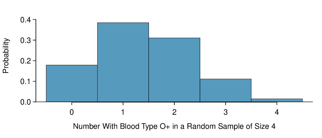
In Example 3.3.6, we asked various probability questions regarding the number of people out of 4 with blood type O+. We verified that the scenario was binomial and that each problem could be solved using the binomial formula. Instead of looking at it piecewise, we could describe the entire distribution of possible values and their corresponding probabilities. Since there are 4 people, there are several possible outcomes for the number who might have blood type O+: 0, 1, 2, 3, 4. We can make a distribution table with these outcomes. Recall that the probability of a randomly sampled person being blood type O+ is about 0.35.
| \(x_i\) | \(P(x_i)\) |
| 0 | \({4\choose 0}(0.35)^0(0.65)^{4} = 0.179\) |
| 1 | \({4\choose 1}(0.35)^1(0.65)^{3} = 0.384\) |
| 2 | \({4\choose 2}(0.35)^2(0.65)^{2} = 0.311\) |
| 3 | \({4\choose 3}(0.35)^3(0.65)^{1} = 0.111\) |
| 4 | \({4\choose 4}(0.35)^4(0.65)^{0} = 0.015\) |
Subsection 4.4.3 The mean and standard deviation of a binomial distribution
Since this is a probability distribution we could find its mean and standard deviation using the formulas from Chapter 3. Those formulas require a lot of calculations, so it is fortunate there's an easier way to compute the mean and standard deviation for a binomial random variable.
Mean and standard deviation of the binomial distribution.
For a binomial distribution with parameters \(n\) and \(p\text{,}\) where \(n\) is the number of trials and \(p\) is the probability of a success, the mean and standard deviation of the number of observed successes are
Example 4.4.2.
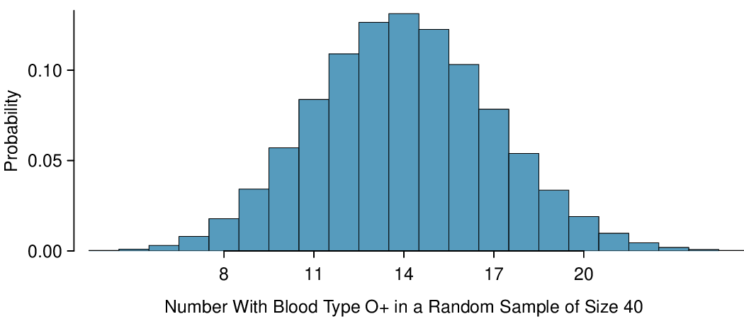
If the probability that a person has blood type O+ is 0.35 and you have 40 randomly selected people, about how many would you expect to have blood type O+? What is the standard deviation of the number of people who would have blood type O+ among the 40 people?
We are asked to determine the expected number (the mean) and the standard deviation, both of which can be directly computed from the formulas above.
The exact distribution is shown in Figure 4.4.3.
Subsection 4.4.4 Normal approximation to the binomial distribution
The binomial formula is cumbersome when the sample size (\(n\)) is large, particularly when we consider a range of observations.
Example 4.4.4.
Find the probability that fewer than 12 out of 40 randomly selected people would have blood type O+, where probability of blood type O+ is 0.35.
This is equivalent to asking, what is the probability of observing \(X=0, 1, 2, ..., \text{ or } 11\) with blood type O+ in a sample of size 40 when \(p=0.35\text{?}\) We previously verified that this scenario is binomial. We can compute each of the 12 probabilities using the binomial formula and add them together to find the answer:
If the true proportion with blood type O+ in the population is \(p = 0.35\text{,}\) then the probability of observing fewer than 12 in a sample of \(n = 40\) is 0.21.
The computations in Example 4.4.4 are tedious and long. In general, we should avoid such work if an alternative method exists that is faster, easier, and still accurate. Recall that calculating probabilities of a range of values is much easier in the normal model. In some cases we may use the normal distribution to estimate binomial probabilities. While a normal approximation for the distribution in Figure 4.4.1 when the sample size was \(n = 4\) would not be appropriate, it might not be too bad for the distribution in Figure 4.4.3 where \(n = 40\text{.}\) We might wonder, when is it reasonable to use the normal model to approximate a binomial distribution?
Checkpoint 4.4.5.
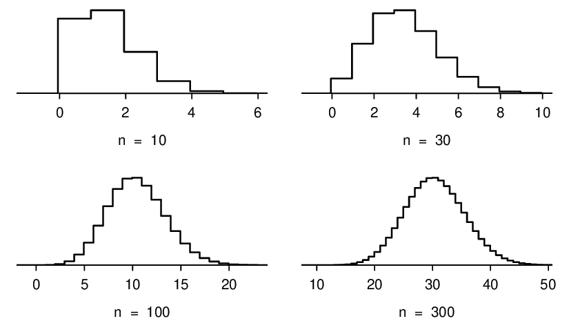
Here we consider the binomial model when the probability of a success is \(p=0.10\text{.}\) Figure 4.4.6 shows four hollow histograms for simulated samples from the binomial distribution using four different sample sizes: \(n=10, 30, 100, 300\text{.}\) What happens to the shape of the distributions as the sample size increases? How does the binomial distribution change as \(n\) gets larger? 1
The shape of the binomial distribution depends upon both \(n\) and \(p\text{.}\) Here we introduce a rule of thumb for when normal approximation of a binomial distribution is reasonable. We will use this rule of thumb in many applications going forward.
Normal approximation of the binomial distribution.
The binomial distribution with probability of success \(p\) is nearly normal when the sample size \(n\) is sufficiently large that \(np\ge 10\) and \(n(1-p)\ge 10\text{.}\) The approximate normal distribution has parameters corresponding to the mean and standard deviation of the binomial distribution:
The normal approximation may be used when computing the range of many possible successes. For instance, we may apply the normal distribution to the setting described in Figure 4.4.3.
Example 4.4.7.
Use the normal approximation to estimate the probability of observing fewer than 12 with blood type O+ in a random sample of 40, if the true proportion with blood type O+ in the population is \(p=0.35\text{.}\)
First we verify that \(np\) and \(n(1-p)\) are at least 10 so that we can apply the normal approximation to the binomial model:
With these conditions checked, we may use the normal distribution to approximate the binomial distribution with the following mean and standard deviation:
We want to find the probability of observing fewer than 12 with blood type O+ using this model. We note that 12 is less than 1 standard deviation below the mean:
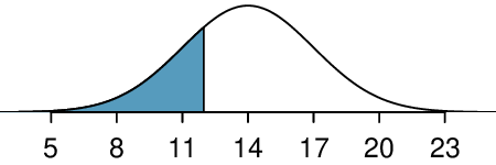
Next, we compute the Z-score as \(Z=\frac{12 - 14}{3} = -0.67\) to find the shaded area in the picture: \(P(Z \lt -0.67) = 0.25\text{.}\) This probability of 0.25 using the normal approximation is reasonably close to the true probability of 0.21 computed using the binomial distribution.
Example 4.4.8.
Use the normal approximation to estimate the probability of observing fewer than 120 people with blood type O+ in a random sample of 400, if the true proportion with blood type O+ in the population is \(p=0.35\text{.}\)
We have previously verified that the binomial model is reasonable for this context. Now we will verify that both \(np\) and \(n(1-p)\) are at least 10 so we can apply the normal approximation to the binomial model:
With these conditions checked, we may use the normal approximation in place of the binomial distribution with the following mean and standard deviation:
We want to find the probability of observing fewer than 120 with blood type O+ using this model. We note that 120 is just over 2 standard deviations below the mean:
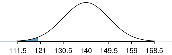
Next, we compute the Z-score as \(Z=\frac{120 - 140}{9.5} = -2.1\) to find the shaded area in the picture: \(P(Z \lt -2.1) = 0.0179\text{.}\) This probability of 0.0179 using the normal approximation is very close to the true probability of 0.0196 from the binomial distribution.
Checkpoint 4.4.9.
Use normal approximation, if applicable, to estimate the probability of getting greater than 15 sixes in 100 rolls of a fair die. 2
Subsection 4.4.5 Normal approximation breaks down on small intervals (special topic)
The normal approximation may fail on small intervals.
The normal approximation to the binomial distribution tends to perform poorly when estimating the probability of a small range of counts, even when the conditions are met.
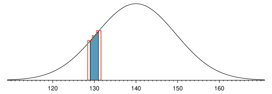
We consider again our example where 35% of people are blood type O+. Suppose we want to find the probability that between 129 and 131 people, inclusive, have blood type O+ in a random sample of 400 people. We want to compute the probability of observing 129, 130, or 131 people with blood type O+ when \(p=0.20\) and \(n=400\text{.}\) With such a large sample, we might be tempted to apply the normal approximation and use the range 129 to 131. However, we would find that the binomial solution and the normal approximation notably differ:
We can identify the cause of this discrepancy using Figure 4.4.10, which shows the areas representing the binomial probability (outlined) and normal approximation (shaded). Notice that the width of the area under the normal distribution is 0.5 units too slim on both sides of the interval. The binomial distribution is a discrete distribution, and the each bar is centered over an integer value. Looking closely at Figure 4.4.10, we can see that the bar corresponding to 129 begins at 128.5 and ends at 129.5, the bar corresponding to 131 begins at 130.5 and ends at 131.5, etc.
Improving accuracy of the normal approximation to the binomial distribution.
The normal approximation to the binomial distribution for intervals of values is usually improved if cutoff values for the lower end of a shaded region are reduced by 0.5 and the cutoff value for the upper end are increased by 0.5. This correction is called the continuity correction and accounts for the fact that the binomial distribution is discrete.
Example 4.4.11.
Use the method described to find a more accurate estimate for the probability of observing 129, 130, or 131 people with blood type O+ in 400 randomly selected people when \(p=0.35\text{.}\)
Instead of standardizing 129 and 131, we will standardize 128.5 and 131.5:
The probability 0.0772 is much closer to the true value of 0.0732 than the previous estimate of 0.0483 we calculated using normal approximation without the continuity correction.
It is always possible to apply the continuity correction when finding a normal approximation to the binomial distribution. However, when \(n\) is very large or when the interval is wide, the benefit of the modification is limited since the added area becomes negligible compared to the overall area being calculated.
Subsection 4.4.6 Section summary
In the previous chapter, we introduced the binomial formula to find the probability of exactly \(x\) successes in \(n\) trials for an event that has probability \(p\) of success. Instead of looking at this scenario piecewise, we can describe the entire distribution of the number of successes and their corresponding probabilities.
The distribution of the number of successes in \(n\) independent trials gives rise to a binomial distribution. If X has a binomial distribution with parameters \(n\) and \(p\text{,}\) then \(P(X=x) = {n\choose x}p^x(1-p)^n-x\text{,}\) where \(x=0,1,2,3\dots,n\text{.}\)
To write out a binomial probability distribution table, list all possible values for \(x\text{,}\) the number of successes, then use the binomial formula to find the probability of each of those values.
Because a binomial distribution can be thought of as the sum of a bunch of 0s and 1s, the Central Limit Theorem applies. As \(n\) gets larger, the shape of the binomial distribution becomes more normal.
We call the rule of thumb for when the binomial distribution can be well modeled with a normal distribution the success-failure condition. The success-failure condition is met when there are at least 10 successes and 10 failures, or when \(np\ge 10\) and \(n(1-p)\ge 10\text{.}\)
-
If X follows a binomial distribution with parameters \(n\) and \(p\text{,}\) then:
The mean is given by \(\mu_{\scriptscriptstyle{X}} = np\text{.}\) (center)
The standard deviation is given by \(\sigma_{\scriptscriptstyle{X}} = \sqrt{np(1-p)}\text{.}\) (spread)
When \(np\ge 10\) and \(n(1-p)\ge 10\text{,}\) the binomial distribution is approximately normal. (shape)
-
It is often easier to use normal approximation to the binomial distribution rather than evaluate the binomial formula many times. These three properties of the binomial distribution are used when solving the following type of problem. Find the probability of getting more than / fewer than x yeses in \(n\) trials or in a sample of size \(n\).
Identify \(n\) and \(p\text{.}\) Verify than \(np\ge 10\) and \(n(1-p)\ge 10\text{,}\) which implies that normal approximation is reasonable.
Calculate the Z-score. Use \(\mu_{\scriptscriptstyle{X}} = np\) and \(\sigma_{\scriptscriptstyle{X}} = \sqrt{np(1-p)}\) to standardize the \(x\) value.
Find the appropriate area under the normal curve.
Exercises 4.4.7 Exercises
1. Underage drinking, Part II.
We learned in Exercise 3.3.6.3 that about 70% of 18-20 year olds consumed alcoholic beverages in any given year. We now consider a random sample of fifty 18-20 year olds.
How many people would you expect to have consumed alcoholic beverages? And with what standard deviation?
Would you be surprised if there were 45 or more people who have consumed alcoholic beverages?
What is the probability that 45 or more people in this sample have consumed alcoholic beverages? How does this probability relate to your answer to part (b)?
(a) \(\mu = 35\text{,}\) \(\sigma = 3.24\text{.}\)
(b) Yes. \(Z = 3.09\text{.}\) Since 45 is more than 2 standard deviations from the mean, it would be considered unusual. Note that the normal model is not required to apply this rule of thumb.
(c) Using a normal model: 0.0010. This does indeed appear to be an unusual observation. If using a normal model with a 0.5 correction, the probability would be calculated as 0.0017.
2. Chickenpox, Part II.
We learned in Exercise 3.3.6.4 that about 90% of American adults had chickenpox before adulthood. We now consider a random sample of 120 American adults.
How many people in this sample would you expect to have had chickenpox in their childhood? And with what standard deviation?
Would you be surprised if there were 105 people who have had chickenpox in their childhood?
What is the probability that 105 or fewer people in this sample have had chickenpox in their childhood? How does this probability relate to your answer to part (b)?
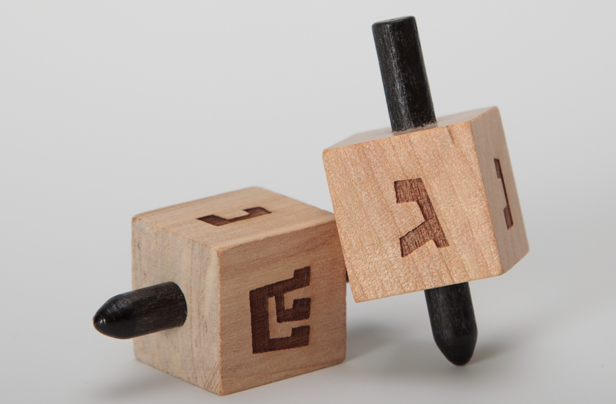
3. Game of dreidel.
A dreidel is a four-sided spinning top with the Hebrew letters nun, gimel, hei, and shin, one on each side. Each side is equally likely to come up in a single spin of the dreidel. Suppose you spin a dreidel three times. Calculate the probability of getting
at least one nun?
exactly 2 nuns?
exactly 1 hei?
at most 2 gimels?
(a) \(1-0.75^3=0.5781\text{.}\)
(b) 0.1406.
(c) 0.4219.
(d) \(1-0.25^3=0.9844\text{.}\)
4. Sickle cell anemia.
Sickle cell anemia is a genetic blood disorder where red blood cells lose their flexibility and assume an abnormal, rigid, “sickle” shape, which results in a risk of various complications. If both parents are carriers of the disease, then a child has a 25% chance of having the disease, 50% chance of being a carrier, and 25% chance of neither having the disease nor being a carrier. If two parents who are carriers of the disease have 3 children, what is the probability that
two will have the disease?
none will have the disease?
at least one will neither have the disease nor be a carrier?
the first child with the disease will the be \(3^{rd}\) child?