
Section 6.4 Chi-square tests for two-way tables
¶We encounter two-way tables in this section, and we learn about two new and closely related chi-square tests. We will answer questions such as the following:
Does the phrasing of the question affect how likely sellers are to disclose problems with a product?
Is gender associated with whether Facebook users know how to adjust their privacy settings?
Is political affiliation associated with support for the use of full body scans at airports?
Subsection 6.4.1 Learning objectives
Calculate the expected counts and degrees of freedom for a chi-square test involving a two-way table.
State and verify whether or not the conditions for a chi-square test for a two-way table are met.
Explain the difference between the chi-square test of homogeneity and chi-square test of independence.
Carry out a complete hypothesis test for homogeneity and for independence.
Subsection 6.4.2 Introduction
Google is constantly running experiments to test new search algorithms. For example, Google might test three algorithms using a sample of 10,000 google.com search queries. Table 6.4.1 shows an example of 10,000 queries split into three algorithm groups. 1 The group sizes were specified before the start of the experiment to be 5000 for the current algorithm and 2500 for each test algorithm.
| Search algorithm | current | test 1 | test 2 | Total | ||
| Counts | 5000 | 2500 | 2500 | 10000 | ||
Example 6.4.2.
What is the ultimate goal of the Google experiment? What are the null and alternative hypotheses, in regular words?
The ultimate goal is to see whether there is a difference in the performance of the algorithms. The hypotheses can be described as the following:
\(H_{0}\text{:}\) The algorithms each perform equally well.
\(H_{A}\text{:}\) The algorithms do not perform equally well.
In this experiment, the explanatory variable is the search algorithm. However, an outcome variable is also needed. This outcome variable should somehow reflect whether the search results align with the user's interests. One possible way to quantify this is to determine whether (1) there was no new, related search, and the user clicked one of the links provided, or (2) there was a new, related search performed by the user. Under scenario (1), we might think that the user was satisfied with the search results. Under scenario (2), the search results probably were not relevant, so the user tried a second search.
Table 6.4.3 provides the results from the experiment. These data are very similar to the count data in Section 6.3. However, now the different combinations of two variables are binned in a two-way table. In examining these data, we want to evaluate whether there is strong evidence that at least one algorithm is performing better than the others. To do so, we apply a chi-square test to this two-way table. The ideas of this test are similar to those ideas in the one-way table case. However, degrees of freedom and expected counts are computed a little differently than before.
| Search algorithm | ||||||
| current | test 1 | test 2 | Total | |||
| No new search | 3511 | 1749 | 1818 | 7078 | ||
| New search | 1489 | 751 | 682 | 2922 | ||
| Total | 5000 | 2500 | 2500 | 10000 | ||
What is so different about one-way tables and two-way tables?
A one-way table describes counts for each outcome in a single variable. A two-way table describes counts for combinations of outcomes for two variables. When we consider a two-way table, we often would like to know, are these variables related in any way?
The hypothesis test for this Google experiment is really about assessing whether there is statistically significant evidence that the choice of the algorithm affects whether a user performs a second search. In other words, the goal is to check whether the three search algorithms perform differently.
Subsection 6.4.3 Expected counts in two-way tables
Example 6.4.4.
From the experiment, we estimate the proportion of users who were satisfied with their initial search (no new search) as \(7078/10000 = 0.7078\text{.}\) If there really is no difference among the algorithms and 70.78% of people are satisfied with the search results, how many of the 5000 people in the “current algorithm” group would be expected to not perform a new search?
About 70.78% of the 5000 would be satisfied with the initial search:
That is, if there was no difference between the three groups, then we would expect 3539 of the current algorithm users not to perform a new search.
Checkpoint 6.4.5.
Using the same rationale described in Solution 6.4.4.1, about how many users in each test group would not perform a new search if the algorithms were equally helpful? 2
We can compute the expected number of users who would perform a new search for each group using the same strategy employed in Solution 6.4.4.1 and Checkpoint 6.4.5. These expected counts were used to construct Table 6.4.6, which is the same as Table 6.4.3, except now the expected counts have been added in parentheses.
| Search algorithm | current | test 1 | test 2 | Total | ||||||
| No new search | 3511 | (3539) | 1749 | (1769.5) | 1818 | (1769.5) | 7078 | |||
| New search | 1489 | (1461) | 751 | (730.5) | 682 | (730.5) | 2922 | |||
| Total | 5000 | 2500 | 2500 | 10000 | ||||||
The examples and exercises above provided some help in computing expected counts. In general, expected counts for a two-way table may be computed using the row totals, column totals, and the table total. For instance, if there was no difference between the groups, then about 70.78% of each column should be in the first row:
Looking back to how the fraction 0.7078 was computed — as the fraction of users who did not perform a new search (\(7078/10000\)) — these three expected counts could have been computed as
This leads us to a general formula for computing expected counts in a two-way table when we would like to test whether there is strong evidence of an association between the column variable and row variable.
Computing expected counts in a two-way table.
To identify the expected count for the \(i^{th}\) row and \(j^{th}\) column, compute
Subsection 6.4.4 The chi-square test of homogeneity for two-way tables
The chi-square test statistic for a two-way table is found the same way it is found for a one-way table. For each table count, compute
Adding the computed value for each cell gives the chi-square test statistic \(\chi^2\text{:}\)
Just like before, this test statistic follows a chi-square distribution. However, the degrees of freedom is computed a little differently for a two-way table. 3 For two way tables, the degrees of freedom is equal to
In our example, the degrees of freedom is
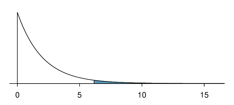
If the null hypothesis is true (i.e. the algorithms are equally useful), then the test statistic \(\chi^2 = 6.12\) closely follows a chi-square distribution with 2 degrees of freedom. Using this information, we can compute the p-value for the test, which is depicted in Figure 6.4.7.
Computing degrees of freedom for a two-way table.
When using the chi-square test to a two-way table, we use
where \(R\) is the number of rows in the table and \(C\) is the number of columns.
Use two-proportion methods for 2-by-2 contingency tables.
When analyzing 2-by-2 contingency tables, use the two-proportion methods introduced in Section 6.2.
Conditions for the chi-square test of homogeneity.
There are two conditions that must be checked before performing a chi-square test of homogeneity. If these conditions are not met, this test should not be used.
Multiple random samples or randomly assigned treatments. Data collected by multiple independent random samples or multiple randomly assigned treatments. Data can then be organized into a two-way table.
All expected counts at least 5. All of the cells in the two-way table must have at least 5 expected cases under the assumption that the null hypothesis is true.
Example 6.4.8.
Compute the p-value and draw a conclusion about whether the search algorithms have different performances.
Here, found that the degrees of freedom for this \(3\times 2\) table is 2. The p-value corresponds to the area under the chi-square curve with 2 degrees of freedom to the right of \(\chi^2=6.120\text{.}\) Using a calculator, we find that the p-value = 0.047. Using an \(\alpha=0.05\) significance level, we reject \(H_0\text{.}\) That is, the data provide convincing evidence that there is some difference in performance among the algorithms.
Notice that the conclusion of the test is that there is some difference in performance among the algorithms. This chi-square test does not tell us which algorithm performed better than the others. To answer this question, we could compare the relevant proportions or construct bar graphs. The proportion that resulted in the new search can be calculated as
This suggests that the current algorithm and test 1 algorithm performed better than the test 2 algorithm; however, to formally test this specific claim we would need to use a test that includes a multiple comparisons correction, which is beyond the scope of this textbook.
A careful reader may have noticed that when there are exactly 2 random samples or treatments and the counts can be arranged in a \(2\times 2\) table, both a chi-square test for homogeneity and a 2-proportion Z-test could apply. In this case, the chi-square test for homogeneity and the two-sided 2-proportion Z-test are equivalent, meaning that they produce the same p-value. 4
\(\chi^2\) test of homogeneity.
When there are multiple samples or treatments and we are comparing the distribution of a categorical variable across several groups, e.g. comparing the distribution of rural/urban/suburban dwellers among 4 states,
Identify: Identify the hypotheses and the significance level, \(\alpha\text{.}\)
\(H_0\text{:}\) The distribution of [...] is the same for each population/treatment.
\(H_A\text{:}\) The distribution of [...] is not the same for each population/treatment.
Choose: Choose the correct test procedure and identify it by name.
Here we choose the \(\chi^2\) test of homogeneity.
Check: Check that the test statistic follows a chi-square distribution.
Data come from multiple random samples or from multiple randomly assigned treatments.
All expected counts are \(\ge 5\) (calculate and record expected counts).
Calculate: Calculate the \(\chi^2\)-statistic, \(df\text{,}\) and p-value.
test statistic: \(\chi^2 =\sum{ \frac{\text{ (observed } - \text{ expected } )^2}{\text{ expected } }}\)
\(df = (\# \text{ of rows } - 1) \times (\# \text{ of columns } - 1)\)
p-value = (area to the right of \(\chi^2\)-statistic with the appropriate \(df\))
Conclude: Compare the p-value to \(\alpha\text{,}\) and draw a conclusion in context.
If the p-value is \(\lt \alpha\text{,}\) reject \(H_0\text{;}\) there is sufficient evidence that [\(H_A\) in context].
If the p-value is \(> \alpha\text{,}\) do not reject \(H_0\text{;}\) there is not sufficient evidence that [\(H_A\) in context].
Example 6.4.9.
In an experiment 5 , each individual was asked to be a seller of an iPod (a product commonly used to store music on before smart phones). The participant received $10 + 5% of the sale price for participating. The iPod they were selling had frozen twice in the past inexplicitly but otherwise worked fine. Unbeknownst to the participants who were the sellers in the study, the buyers were collaborating with the researchers to evaluate the influence of different questions on the likelihood of getting the sellers to disclose the past issues with the iPod. The scripted buyers started with “Okay, I guess I'm supposed to go first. So you've had the iPod for 2 years ...” and ended with one of three questions:
General: What can you tell me about it?
Positive Assumption: It doesn't have any problems, does it?
Negative Assumption: What problems does it have?
The outcome variable is whether the participant discloses or hides the problem with the iPod.
| Question Type | ||||
| General | Positive Assump. | Negative Assump. | ||
| Response | Disclose | 2 | 23 | 36 |
| Hide | 71 | 50 | 37 | |
| Total | 73 | 73 | 73 | |
Does the phrasing of the question affect how likely individuals are to disclose the problems with the iPod? Carry out an appropriate test at the 0.05 significance level.
Identify: We will test the following hypotheses at the \(\alpha=0.05\) significance level.
\(H_0\text{:}\) The likelihood of disclosing the problem is the same for each question type.
\(H_A\text{:}\) The likelihood of disclosing the problem is not the same for each question type.
Choose: We want to know if the distribution of disclose/hide is the same for each of the three question types, so we want to carry out a chi-square test for homogeneity.
Check: This is an experiment in which there were three randomly allocated treatments. Here a treatment corresponds to a question type. All values in the table of expected counts are \(\ge\) 5. Table of expected counts:
| Question Type | ||||
| General | Positive Assump. | Negative Assump. | ||
| Response | Disclose | 20.3 | 20.3 | 20.3 |
| Hide | 52.7 | 52.7 | 52.7 | |
| Total | 73 | 73 | 73 | |
Calculate: Using technology, we get \(\chi^2 = 40.1\)
\(df = (\# \text{ of rows } - 1) \times (\# \text{ of columns } - 1) = 2\times 1 = 2\)
The p-value is the area under the chi-square curve with 2 degrees of freedom to the right of \(\chi^2=40.1\text{.}\) Thus, the p-value is almost 0.
Conclude: Because the p-value \(\approx\) 0 \(\lt \alpha\text{,}\) we reject \(H_0\text{.}\) We have strong evidence that the likelihood of disclosing the problem is not the same for each question type.
Checkpoint 6.4.10.
If an error was made in the test in the previous example, would it have been a Type I error or a Type II error? 6
Subsection 6.4.5 The chi-square test of independence for two-way tables
Often, instead of having separate random samples or treatments, we have just one sample and we want to look at the association between two variables. When these two variables are categorical, we can arrange the responses in a two-way table.
In Chapter 3 we looked at independence in the context of probability. Here we look at independence in the context of inference. We want to know if any observed association is due to random chance or if there is evidence of a real association in the population that the sample was taken from. To answer this, we use a chi-square test for independence. The chi-square test of independence applies when there is only one random sample and there are two categorical variables. The null claim is always that the two variables are independent, while the alternate claim is that the variables are dependent.
Example 6.4.11.
Table 6.4.12 summarizes the results of a Pew Research poll 7 . A random sample of adults in the U.S. was taken, and each was asked whether they approved or disapproved of the job being done by President Obama, Democrats in Congress, and Republicans in Congress. The results are shown in Table 6.4.12. We would like to determine if the three groups and the approval ratings are associated. What are appropriate hypotheses for such a test?
\(H_{0}\) The group and their ratings are independent. (There is no difference in approval ratings between the three groups.)
\(H_{A}\) The group and their ratings are dependent. (There is some difference in approval ratings between the three groups, e.g. perhaps Obama's approval differs from Democrats in Congress.)
| Congress | ||||||
| Obama | Democrats | Republicans | Total | |||
| Approve | 842 | 736 | 541 | 2119 | ||
| Disapprove | 616 | 646 | 842 | 2104 | ||
| Total | 1458 | 1382 | 1383 | 4223 | ||
Conditions for the chi-square test of independence.
There are two conditions that must be checked before performing a chi-square test of independence. If these conditions are not met, this test should not be used.
One random sample with two variables/questions. The data must be arrived at by taking a random sample.After the data is collected, it is separated and categorized according to two variables and can be organized into a two-way table.
All expected counts at least 5. All of the cells in the two-way table must have at least 5 expected cases assuming the null hypothesis is true.
Example 6.4.13.
First, we observe that the data came from a random sample of adults in the U.S. Next, let's compute the expected values that correspond to Table 6.4.12, if the null hypothesis is true, that is, if group and rating are independent.
The expected count for row one, column one is found by multiplying the row one total (2119) and column one total (1458), then dividing by the table total (4223): \(\frac{2119\times 1458}{4223} = 731.6\text{.}\) Similarly for the first column and the second row: \(\frac{2104\times 1458}{4223} = 726.4\text{.}\) Repeating this process, we get the expected counts:
| Obama | Congr. Dem. | Congr. Rep. | |
| Approve | 731.6 | 693.5 | 694.0 |
| Disapprove | 726.4 | 688.5 | 689.0 |
The table above gives us the number we would expect for each of the six combinations if group and rating were really independent. Because all of the expected counts are at least 5 and there is one random sample, we can carry out the chi-square test for independence.
The chi-square test of independence and the chi-square test of homogeneity both involve counts in a two-way table. The chi-square statistic and the degrees of freedom are calculated in the same way.
Example 6.4.14.
Calculate the chi-square statistic.
We calculate \(\frac{(\text{ obs } - \text{ exp } )^2}{\text{ exp } }\) for each of the six cells in the table. Adding the results of each cell gives the chi-square test statistic.
Example 6.4.15.
Find the p-value for the test and state the appropriate conclusion.
We must first find the degrees of freedom for this chi-square test. Because there are 2 rows and 3 columns, the degrees of freedom is \(df=(2-1)\times (3-1) = 2\text{.}\) We find the area to the right of \(\chi^2=106.4\) under the chi-square curve with \(df=2\text{.}\) The p-value is extremely small, much less than 0.01, so we reject \(H_0\text{.}\) We have evidence that the three groups and their approval ratings are dependent.
\(\chi^2\) test of independence.
When there is one sample and we are looking for association or dependence between two categorical variables, e.g. testing for an association between gender and political party,
Identify: Identify the hypotheses and the significance level, \(\alpha\text{.}\)
\(H_0\text{:}\) [variable 1] and [variable 2] are independent.
\(H_A\text{:}\) [variable 1] and [variable 2] are dependent.
Choose: Choose the correct test procedure and identify it by name.
Here we choose the \(\chi^2\) test of independence.
Check: Check that the test statistic follows a chi-square distribution.
Data come from a single random sample.
All expected counts are \(\ge 5\) (calculate and record expected counts).
Calculate: Calculate the \(\chi^2\)-statistic, \(df\text{,}\) and p-value.
test statistic: \(\chi^2 =\sum{ \frac{\text{ (observed } - \text{ expected } )^2}{\text{ expected } }}\)
\(df = (\# \text{ of rows } - 1) \times (\# \text{ of columns } - 1)\)
p-value = (area to the right of \(\chi^2\)-statistic with the appropriate \(df\))
Conclude: Compare the p-value to \(\alpha\text{,}\) and draw a conclusion in context.
If the p-value is \(\lt \alpha\text{,}\) reject \(H_0\text{;}\) there is sufficient evidence that [\(H_A\) in context].
If the p-value is \(> \alpha\text{,}\) do not reject \(H_0\text{;}\) there is not sufficient evidence that [\(H_A\) in context].
Example 6.4.16.
A 2011 survey asked 806 randomly sampled adult Facebook users about their Facebook privacy settings. One of the questions on the survey was, “Do you know how to adjust your Facebook privacy settings to control what people can and cannot see?” The responses are cross-tabulated based on gender.
| Gender | ||||
| Male | Female | Total | ||
| Response | Yes | 288 | 378 | 666 |
| No | 61 | 62 | 123 | |
| Not sure | 10 | 7 | 17 | |
| Total | 359 | 447 | 806 | |
Carry out an appropriate test at the 0.10 significance level to see if there is an association between gender and knowing how to adjust Facebook privacy settings to control what people can and cannot see.
Identify: We will test the following hypotheses at the \(\alpha=0.10\) significance level.
\(H_0\text{:}\) Gender and knowing how to adjust Facebook privacy settings are independent.
\(H_A\text{:}\) Gender and knowing how to adjust Facebook privacy settings are dependent.
Choose: Two variables were recorded on the respondents: gender and response to the question regarding privacy settings. We want to know if these variables are associated / dependent, so we will carry out a chi-square test of independence.
Check: According to the problem, there was one random sample taken. All values in the table of expected counts are \(\ge\) 5. Table of expected counts:
| Gender | |||
| Male | Female | ||
| Response | Yes | 296.64 | 369.36 |
| No | 54.785 | 68.215 | |
| Not sure | 7.572 | 9.428 | |
Calculate: Using technology, we get \(\chi^2 = 3.13\text{.}\) The degrees of freedom for this test is given by: \(df = (\# \text{ of rows } - 1) \times (\# \text{ of columns } - 1) = 2\times 1 = 2\)
The p-value is the area under the chi-square curve with 2 degrees of freedom to the right of \(\chi^2=3.13\text{.}\) Thus, the p-value = 0.209.
Conclude: Because the p-value = 0.209 \(> \alpha\text{,}\) we do not reject \(H_0\text{.}\) We do not have sufficient evidence that gender and knowing how to adjust Facebook privacy settings are dependent.
Checkpoint 6.4.17.
In context, interpret the p-value of the test in the previous example. 8
Subsection 6.4.6 Calculator: chi-square test for two-way tables
¶TI-83/84: Entering data into a two-way table.
Hit
2ND\(x^{-1}\) (i.e.MATRIX).Right arrow to
EDIT.Hit
1orENTERto select matrixA.Enter the dimensions by typing #rows,
ENTER, #columns,ENTER.Enter the data from the two-way table.
Chi-square test of homogeneity and independence.
Use STAT, TESTS, \(\chi^2\)-Test.
First enter two-way table data as described in the previous box.
Choose
STAT.Right arrow to
TESTS.Down arrow and choose
C:\(\chi^2\)-Test.-
Down arrow, choose
Calculate, and hitENTER, which returns\(\chi^2\) chi-square test statistic pp-value dfdegrees of freedom
Chi-square test of homogeneity and independence.
TI-83/84: Finding the expected counts
First enter two-way table data as described previously.
Carry out the chi-square test of homogeneity or independence as described in previous box.
Hit
2ND\(x^{-1}\) (i.e.MATRIX).Right arrow to
EDIT.Hit
2to see matrixB. This matrix contains the expected counts.
Casio fx-9750GII: Chi-square test of homogeneity and independence.
Navigate to
STAT(MENUbutton, then hit the2button or selectSTAT).Choose the
TESToption (F3button).Choose the
CHIoption (F3button).Choose the
2WAYoption (F2button).-
Enter the data into a matrix:
Hit \(\triangleright\)
MAT(F2button).Navigate to a matrix you would like to use (e.g.
Mat C) and hitEXE.Specify the matrix dimensions:
mis for rows,nis for columns.Enter the data.
Return to the test page by hitting
EXITtwice.
Enter the
Observedmatrix that was used by hittingMAT(F1button) and the matrix letter (e.g.C).Enter the
Expectedmatrix where the expected values will be stored (e.g.D).-
Hit the
EXEbutton, which returns\(\chi^2\) chi-square test statistic pp-value dfdegrees of freedom To see the expected values of the matrix, go to \(\triangleright\)
MAT(F6button) and select the corresponding matrix.
Checkpoint 6.4.18.
Use Table 6.4.12, reproduced below, and a calculator to find the expected values and the \(\chi^2\)-statistic, \(df\text{,}\) and p-value for the chi-square test for independence.
| Congress | ||||||
| Obama | Democrats | Republicans | Total | |||
| Approve | 842 | 736 | 541 | 2119 | ||
| Disapprove | 616 | 646 | 842 | 2104 | ||
| Total | 1458 | 1382 | 1383 | 4223 | ||
Subsection 6.4.7 Section summary
When there are two categorical variables, rather than one, the data must be arranged in a two-way table and a \(\chi^2\) test of homogeneity or a \(\chi^2\) test of independence is appropriate.
These tests use the same \(\chi^2\)-statistic as the chi-square goodness of fit test, but instead of number of categories \(-\) 1, the degrees of freedom is (\(\# \text{ of rows } - 1)\times (\# \text{ of columns } -1\)). All expected counts must be at least 5.
When working with a two-way table, the expected count for each row,column combination is calculated as: expected count = \(\frac{(\text{ row total } )\times (\text{ column total } )}{\text{ table total } }\text{.}\)
The \(\chi^2\) test of homogeneity and the \(\chi^2\) test of independence are almost identical. The differences lie in the data collection method and in the hypotheses.
-
When there are multiple samples or treatments and we are comparing the distribution of a categorical variable across several groups, e.g. comparing the distribution of rural/urban/suburban dwellers among 4 states, the hypotheses can often be written as follows:
\(H_0\text{:}\) The distribution of [...] is the same for each population/treatment.
\(H_A\text{:}\) The distribution of [...] is not the same for each population/treatment.
We test these hypotheses at the \(\alpha\) significance level using a \(\chi^2\) test of homogeneity.
-
When there is one sample and we are looking for association or dependence between two categorical variables, e.g. testing for an association between gender and political party, the hypotheses can be written as:
\(H_0\text{:}\) [variable 1] and [variable 2] are independent.
\(H_A\text{:}\) [variable 1] and [variable 2] are dependent.
We test these hypotheses at the \(\alpha\) significance level using a \(\chi^2\) test of independence.
Both of the \(\chi^2\) tests for two-way tables require that all expected counts are \(\ge\) 5.
-
The chi-square statistic is:
test statistic: \(\chi^2 =\sum{ \frac{\text{ (observed } - \text{ expected } )^2}{\text{ expected } }}\)
\(df =\) (# of rows \(-\) 1)(# of cols \(-\) 1)
The p-value is the area to the right of \(\chi^2\)-statistic under the chi-square curve with the appropriate \(df\text{.}\)
Exercises 6.4.8 Exercises
1. Quitters.
Does being part of a support group affect the ability of people to quit smoking? A county health department enrolled 300 smokers in a randomized experiment. 150 participants were assigned to a group that used a nicotine patch and met weekly with a support group; the other 150 received the patch and did not meet with a support group. At the end of the study, 40 of the participants in the patch plus support group had quit smoking while only 30 smokers had quit in the other group.
Create a two-way table presenting the results of this study.
-
Answer each of the following questions under the null hypothesis that being part of a support group does not affect the ability of people to quit smoking, and indicate whether the expected values are higher or lower than the observed values.
How many subjects in the “patch + support” group would you expect to quit?
How many subjects in the “patch only” group would you expect to not quit?
(a) Two-way table:
| Quit | |||
| Treatment | Yes | No | Total |
| Patch + support group | 40 | 110 | 150 |
| Only patch | 30 | 120 | 150 |
| Total | 70 | 230 | 300 |
(b-i) \(E_{row_{1},col_{1}} = \frac{(row 1 total)\times(col 1 total)}{table total} = 35\text{.}\) This is lower than the observed value.
(b-ii) \(E_{row_{2},col_{2}} = \frac{(row 2 total)\times(col 2 total)}{table total} = 115\text{.}\) This is lower than the observed value.
2. Full body scan, Part II.
The table below summarizes a data set we first encountered in Exercise 6.2.9.10 regarding views on full-body scans and political affiliation. The differences in each political group may be due to chance. Complete the following computations under the null hypothesis of independence between an individual's party affiliation and his support of full-body scans. It may be useful to first add on an extra column for row totals before proceeding with the computations.
| Party Affiliation | ||||
| Republican | Democrat | Independent | ||
| Answer | Should | 264 | 299 | 351 |
| Should not | 38 | 55 | 77 | |
| Don't know/No answer | 16 | 15 | 22 | |
| Total | 318 | 369 | 450 | |
How many Republicans would you expect to not support the use of full-body scans?
How many Democrats would you expect to support the use of full- body scans?
How many Independents would you expect to not know or not answer?
3. Offshore drilling, Part III.
The table below summarizes a data set we first encountered in Exercise 6.2.9.7 that examines the responses of a random sample of college graduates and non-graduates on the topic of oil drilling. Complete a chi-square test for these data to check whether there is a statistically significant difference in responses from college graduates and non-graduates.
| College Grad | ||
| Yes | No | |
| Support | 154 | 132 |
| Oppose | 180 | 126 |
| Do not know | 104 | 131 |
| Total | 438 | 389 |
\(H_{0}:\) The opinion of college grads and non-grads is not different on the topic of drilling for oil and natural gas off the coast of California. \(H_{A}:\) Opinions regarding the drilling for oil and natural gas off the coast of California has an association with earning a college degree.
Independence: The samples are both random, unrelated, and from less than 10% of the population, so independence between observations is reasonable. Sample size: All expected counts are at least 5. \(\chi^2 = 11.47, df = 2 \rightarrow \text{p-value } = 0.003\text{.}\) Since the p-value \(< \sigma\text{,}\) we reject \(H_{0}\text{.}\) There is strong evidence that there is an association between support for off-shore drilling and having a college degree.
4. Parasitic worm.
Lymphatic filariasis is a disease caused by a parasitic worm. Complications of the disease can lead to extreme swelling and other complications. Here we consider results from a randomized experiment that compared three different drug treatment options to clear people of the this parasite, which people are working to eliminate entirely. The results for the second year of the study are given below: 9
| Clear at Year 2 | Not Clear at Year 2 | |
| Three drugs | 52 | 2 |
| Two drugs | 31 | 24 |
| Two drugs annually | 42 | 14 |
Set up hypotheses for evaluating whether there is any difference in the performance of the treatments, and also check conditions.
-
Statistical software was used to run a chi-square test, which output:
\begin{align*} \amp X^2 = 23.7 \amp \amp df = 2 \amp \amp \text{ p-value } = \text{ 7.2e-6 } \end{align*}Use these results to evaluate the hypotheses from part (a), and provide a conclusion in the context of the problem.
Subsection 6.4.9 Chapter Highlights
Calculating a confidence interval or a test statistic and p-value are generally done with statistical software. It is important, then, to focus not on the calculations, but rather on
choosing the correct procedure
understanding when the procedures do or do not apply, and
interpreting the results.
Choosing the correct procedure requires understanding the type of data and the method of data collection. All of the inference procedures in Chapter 6 are for categorical variables. Here we list the five tests encountered in this chapter and when to use them.
-
1-proportion Z-test
1 random sample, a yes/no variable
Compare the sample proportion to a fixed / hypothesized proportion.
-
2-proportion Z-test
2 independent random samples or randomly allocated treatments
Compare two populations or treatments to each other with respect to one yes/no variable; e.g. comparing the proportion over age 65 in two distinct populations.
-
\(\chi^2\) goodness of fit test
1 random sample, a categorical variable (generally at least three categories)
Compare the distribution of a categorical variable to a fixed or known population distribution; e.g. looking at distribution of color among M&M's.
-
\(\chi^2\) test of homogeneity:
2 or more independent random samples or randomly allocated treatments
Compare the distribution of a categorical variable across several populations or treatments; e.g. party affiliation over various years, or patient improvement compared over 3 treatments.
-
\(\chi^2\) test of independence
1 random sample, 2 categorical variables
Determine if, in a single population, there is an association between two categorical variables; e.g. grade level and favorite class.
Even when the data and data collection method correspond to a particular test, we must verify that conditions are met to see if the assumptions of the test are reasonable. All of the inferential procedures of this chapter require some type of random sample or process. In addition, the 1-proportion Z-test/interval and the 2-proportion Z-test/interval require that the success-failure condition is met and the three \(\chi^2\) tests require that all expected counts are at least 5.
Finally, understanding and communicating the logic of a test and being able to accurately interpret a confidence interval or p-value are essential. For a refresher on this, review Chapter 5: Foundations for inference.