Section 4.5 Sampling distribution of a sample proportion
¶Often, instead of the number of successes in \(n\) trials, we are interested in the proportion of successes in \(n\) trials. We can use the sampling distribution of a sample proportion to answer questions such as the following:
Given a population that is 50% male, what is the probability that a random sample of 200 people would consist of less than 45% males?
In a particular state, 48% support a controversial measure. When estimating the percent through polling, what is the probability that a random sample of size 200 will mistakenly estimate the percent support to be greater than 50%?
Subsection 4.5.1 Learning objectives
Describe the center, spread, and shape of the sampling distribution of a sample proportion.
Recognize the relationship between the distribution of a sample proportion and the corresponding binomial distribution.
Identify and explain the conditions for using normal approximation involving a sample proportion. Recognize that the Central Limit Theorem applies in the case of proportions/counts as well as means/sums.
Verify that the conditions for normal approximation are met and carry out normal approximation involving a sample proportion or sample count.
Subsection 4.5.2 The mean and standard deviation of \(\hat{p}\)
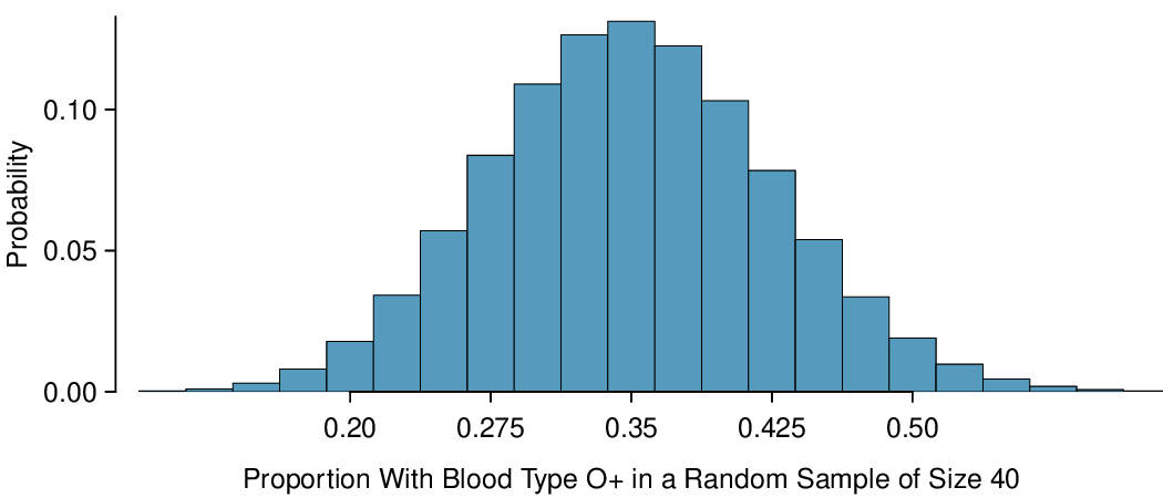
To answer these questions, we investigate the distribution of the sample proportion \(\hat{p}\text{.}\) In the last section we saw that the number of people with blood type O+ in a random sample of size 40 follows a binomial distribution with \(n=40\) and \(p=0.35\) that is centered on 14 and has standard deviation 3.0. What does the distribution of the proportion of people with blood type O+ in a sample of size 40 look like? To convert from a count to a proportion, we divide the count (i.e. number of yeses) by the sample size, \(n = 40\text{.}\) For example, 6 becomes \(8/40 = 0.20\) as a proportion and 11 becomes \(11/40 = 0.275\text{.}\)
We can find the general formula for the mean (expected value) and standard deviation of a sample proportion \(\hat{p}\) using our tools that we've learned so far. To get the sample mean for \(\hat{p}\text{,}\) we divide the binomial mean \(\mu_{binomial} = np\) by \(n\text{:}\)
As one might expect, the sample proportion \(\hat{p}\) is centered on the true proportion \(p\text{.}\) Likewise, the standard deviation of \(\hat{p}\) is equal to the standard deviation of the binomial distribution divided by \(n\text{:}\)
Mean and standard deviation of a sample proportion.
The mean and standard deviation of the sample proportion describe the center and spread of the distribution of all possible sample proportions \(\hat{p}\) from a random sample of size \(n\) with true population proportion \(p\text{.}\)
In analyses, we think of the formula for the standard deviation of a sample proportion, \(\sigma_{\hat{p}}\text{,}\) as describing the uncertainty associated with the estimate \(\hat{p}\text{.}\) That is, \(\sigma_{\hat{p}}\) can be thought of as a way to quantify the typical error in our sample estimate \(\hat{p}\) of the true proportion \(p\text{.}\) Understanding the variability of statistics such as \(\hat{p}\) is a central component in the study of statistics.
Here, \(n=40\) and \(p=0.35\text{,}\) \(\sigma_{\hat{p}} = \sqrt{\frac{0.35(1-0.35)}{40}}=0.075\text{.}\) We see in Figure 4.5.1 that the distribution of number of people in a sample with blood type O+ out of 40 is equivalent to the distribution of proportion of people in a sample of size 40 with blood type O+, but with a change of scale. Instead of counts along the horizontal axis, we have proportions.

Example 4.5.2.
If the proportion of people in the county with blood type O+ is really 35%, find and interpret the mean and standard deviation of the sample proportion for a random sample of size 400.
The mean of the sample proportion is the population proportion: 0.35. That is, if we took many, many samples and calculated \(\hat{p}\text{,}\) these values would average out to \(p = 0.35\text{.}\)
The standard deviation of \(\hat{p}\) is described by the standard deviation for the proportion:
The sample proportion will typically be about 0.024 or 2.4% away from the true proportion of \(p = 0.35\text{.}\) We'll become more rigorous about quantifying how close \(\hat{p}\) will tend to be to \(p\) in Chapter 5.
Subsection 4.5.3 The Central Limit Theorem revisited
In Section 4.2, we saw the Central Limit Theorem, which states that for large enough \(n\text{,}\) the sample mean \(\bar{x}\) is normally distributed.
A natural question is, what does this have to do with sample proportions? In fact, a lot! A sample proportion can be written down as a sample mean. For example, suppose we have 3 successes in 10 trials. If we label each of the 3 success as a 1 and each of the 7 failures as a 0, then the sample proportion is the same as the sample mean:
That is, the distribution of the sample proportion is governed by the Central Limit Theorem, and the Central Limit Theorem is what ties together much of the statistical theory we will see.
Three important facts about the distribution of a sample proportion \(\hat{{p}}\).
Consider taking a simple random sample from a large population.
The mean of a sample proportion is \(p\text{.}\)
The SD of a sample proportion is \(\sqrt{\frac{p(1-p)}{n}}\text{.}\)
When \(np \geq 10\) and \(n(1-p) \geq 10\text{,}\) the sample proportion closely follows a normal distribution.
Using these facts, we can now answer the question posed at the beginning of this section.
Subsection 4.5.4 Normal approximation for the distribution of \(\hat{p}\)
Example 4.5.3.
Find the probability that less than 30% of a random sample of 400 people will be blood type O+ if the population proportion is 35%.
In the previous section we verified that \(np\) and \(n(1-p)\) are at least 10. The mean of the sample proportion is 0.35 and the standard deviation for the sample proportion is given by \(\sqrt{\frac{0.35(1-0.35)}{400}}=0.024\text{.}\) We can find a Z-score and use our calculator to find the probability:
We leave it to the reader to construct a figure for this example.
Example 4.5.4.
The probability 0.0179 is the same probability we calculated when we found the probability of getting fewer than 120 with blood type O+ out of 400! Why is this?
Notice that \(120/400=0.30\text{.}\) Using the binomial distribution to find the probability of fewer than 120 with blood type O+ in the sample is equivalent to using the distribution of \(\hat{p}\) to find the probability of a sample proportion less than 0.30.
Checkpoint 4.5.5.
Given a population that is 50% male, what is the probability that a sample of size 200 would have greater than 55% males? Remember to verify that conditions for normal approximation are met. 1
Subsection 4.5.5 Section summary
The binomial distribution shows the distribution of the number of successes in \(n\) trials. Often, we are interested in the proportion of successes rather than the number of successes.
To convert from "number of yeses" to "proportion of yeses" we simply divide the number by \(n\text{.}\) The sampling distribution of the sample proportion \(\hat{p}\) is identical to the binomial distribution with a change of scale, i.e. different mean and different SD, but same shape.
The same success-failure condition for the binomial distribution holds for a sample proportion \(\hat{p}\text{.}\)
-
Three important facts about the sampling distribution of the sample proportion \(\hat{p}\text{:}\)
The mean of a sample proportion is denoted by \(\mu_{\hat{p}}\text{,}\) and it is equal to \(p\text{.}\) (center)
The SD of a sample proportion is denoted by \(\sigma_{\hat{p}}\text{,}\) and it is equal to \(\sqrt{\frac{p(1-p)}{n}}\text{.}\) (spread)
When \(np\ge 10\) and \(n(1-p)\ge 10\text{,}\) the distribution of the sample proportion will be approximately normal. (shape)
-
We use these properties when solving the following type of normal approximation problem involving a sample proportion. Find the probability of getting more / less than \(x\)% yeses in a sample of size \(n\).
Identify \(n\) and \(p\text{.}\) Verify than \(np\ge 10\) and \(n(1-p)\ge 10\text{,}\) which implies that normal approximation is reasonable.
Calculate the Z-score. Use \(\mu_{\hat{p}} = p\) and \(\sigma_{\hat{p}} = \sqrt{\frac{p(1-p)}{n}}\) to standardize the sample proportion.
Find the appropriate area under the normal curve.
Exercises 4.5.6 Exercises
1. Distribution of \(\hat{p}\).
Suppose the true population proportion were \(p = 0.95\text{.}\) The figure below shows what the distribution of a sample proportion looks like when the sample size is \(n = 20\text{,}\) \(n = 100\text{,}\) and \(n = 500\text{.}\) (a) What does each point (observation) in each of the samples represent? (b) Describe the distribution of the sample proportion, \(\hat{p}\text{.}\) How does the distribution of the sample proportion change as \(n\) becomes larger?
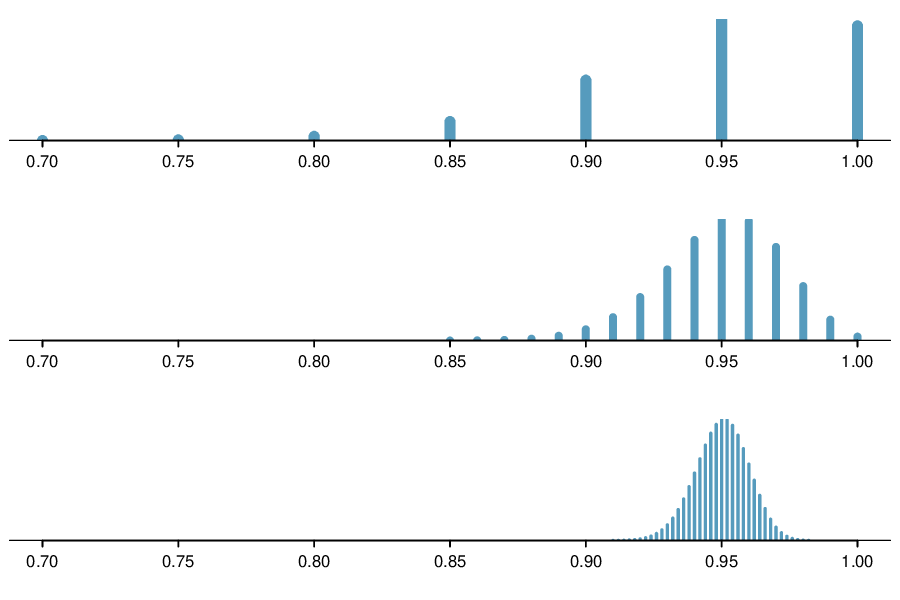
(a) Each observation in each of the distributions represents the sample proportion (\(\hat{p}\)) from samples of size \(n = 20\text{,}\) \(n = 100\text{,}\) and \(n = 500\text{,}\) respectively.
(b) The centers for all three distributions are at 0.95, the true population parameter. When \(n\) is small, the distribution is skewed to the left and not smooth. As n increases, the variability of the distribution (standard deviation) decreases, and the shape of the distribution becomes more unimodal and symmetric.
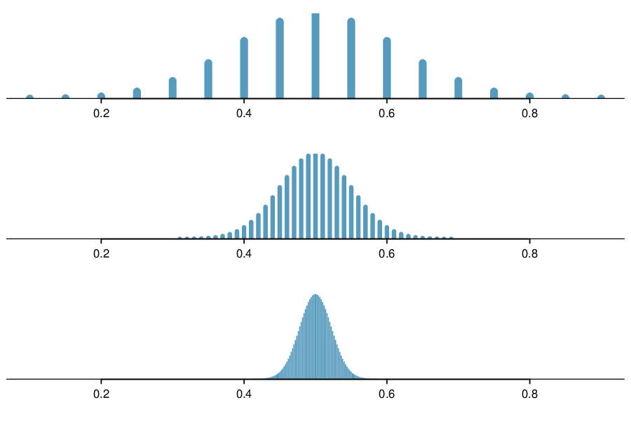
2. Distribution of \(\hat{p}\).
Suppose the true population proportion were \(p = 0.5\text{.}\) The figure below shows what the distribution of a sample proportion looks like when the sample size is \(n = 20\text{,}\) \(n = 100\text{,}\) and \(n = 500\text{.}\) What does each point (observation) in each of the samples represent? Describe how the distribution of the sample proportion, \(\hat{p}\text{,}\) changes as \(n\) becomes larger.
3. Distribution of \(\hat{p}\).
Suppose the true population proportion were \(p = 0.5\) and a researcher takes a simple random sample of size \(n=50\text{.}\)
Find and interpret the standard deviation of the sample proportion \(\hat{p}\text{.}\)
Calculate the probability that the sample proportion will be larger than 0.55 for a random sample of size 50.
(a) \(SD_{\hat{p}} = \sqrt{p(1 - p)/n} = 0.0707\text{.}\) This describes the typical distance that the sample proportion will deviate from the true proportion, \(p = 0.5\text{.}\)
(b) \(\hat{p}\) approximately follows \(N(0.5, 0.0707)\text{.}\) \(Z = (0.55 - 0.50)/0.0707 \approx 0.71\text{.}\) This corresponds to an upper tail of about 0.2389. That is, \(P(\hat{p} > 0.55) \approx 0.24\text{.}\)
4. Distribution of\(\hat{p}\).
Suppose the true population proportion were \(p = 0.6\) and a researcher takes a simple random sample of size \(n=50\text{.}\)
Find and interpret the standard deviation of the sample proportion \(\hat{p}\text{.}\)
Calculate the probability that the sample proportion will be larger than 0.65 for a random sample of size 50.
5. Nearsighted children.
It is believed that nearsightedness affects about 8% of all children. We are interested in finding the probability that fewer than 12 out of 200 randomly sampled children will be nearsighted.
Estimate this probability using the normal approximation to the binomial distribution.
Estimate this probability using the distribution of the sample proportion.
How do your answers from parts (a) and (b) compare?
(a) First we need to check that the necessary conditions are met. There are \(200 \times 0.08 = 16 \) expected successes and \(200 \times (1 - 0.08) = 184\) expected failures, therefore the success-failure condition is met. Then the binomial distribution can be approximated by \(N(\mu = 16, \sigma = 3.84)\text{.}\) \(P(X \lt 12) = P(Z \lt -1.04) = 0.1492\text{.}\)
(b) Since the success-failure condition is met the sampling distribution of \(\hat{p} ~ N(\mu = 0.08, \sigma = 0.0192)\text{.}\) \(P(\hat{p} \lt 0.06)= P(Z \lt -1.04) = 0.1492\)/
(c) As expected, the two answers are the same.
6. Social network use.
The Pew Research Center estimates that as of January 2014, 89% of 18-29 year olds in the United States use social networking sites. 2 Calculate the probability that at least 95% of 500 randomly sampled 18-29 year olds use social networking sites.
Subsection 4.5.7 Chapter Highlights
This chapter began by introducing the normal distribution. A common thread that ran through this chapter is the use of the normal approximation in various contexts. The key steps are included for each of the normal approximation scenarios below.
Normal approximation for data: - Verify that population is approximately normal. - Use the given mean \(\mu\) and SD \(\sigma\) to find the Z-score for the given \(x\) value.
Normal approximation for a sample mean/sum : Verify that population is approximately normal or that \(n\ge 30\text{.}\) Use \(\mu_{\bar{x}}=\mu\) and \(\sigma_{\bar{x}}=\frac{\sigma}{\sqrt{n}}\) to find the Z-score for the given/calculated sample mean.
Normal approximation for the number of successes (binomial): - Verify that \(np\ge 10\) and \(n(1-p)\ge 10\text{.}\) - Use \(\mu_{\scriptscriptstyle{X}} = np\) and \(\sigma_{\scriptscriptstyle{X}} = \sqrt{np(1-p)}\) to find the Z-score for the given number of successes.
Normal approximation for a sample proportion: - Verify that \(np\ge 10\) and \(n(1-p)\ge 10\text{.}\) - Use \(\mu_{\hat{p}} = p\) and \(\sigma_{\hat{p}} = \sqrt{\frac{p(1-p)}{n}}\) to find the Z-score for the given sample proportion.
Normal approximation for the sum of two independent random variables: - Verify that each random variable is approximately normal. - Use \(E(X+Y)=E(X)+E(Y)\) and \(SD(X+Y)=\sqrt{(SD(X))^2+(SD(Y))^2}\) to find the Z-score for the given sum.
Cases 1 and 2 apply to numerical variables, while cases 3 and 4 are for categorical yes/no variables. Case 5 applies to both numerical and categorical variables.
Note that in the binomial case and in the case of proportions, we never look to see if the population is normal. That would not make sense because the “population” is simply a bunch of no/yes, 0/1 values and could not possibly be normal.
The Central Limit Theorem is the mathematical rule that ensures that when the sample size is sufficiently large, the sample mean/sum and sample proportion/count will be approximately normal.