Section 4.1 Normal distribution
¶What proportion of adults have systolic blood pressure above 140? What is the probability of getting more than 250 heads in 400 tosses of a fair coin? If the average weight of a piece of carry-on luggage is 11 pounds, what is the probability that 200 random carry on pieces will weigh more than 2500 pounds? If 55% of a population supports a certain candidate, what is the probability that she will have less than 50% support in a random sample of size 200?
There is one distribution that can help us answer all of these questions. Can you guess what it is? That's right — it's the normal distribution.
Subsection 4.1.1 Learning objectives
Calculate and interpret a Z-score.
Understand that Z-scores are unitless (standard units) and are not affected by change of units.
Use the normal model to approximate a distribution where appropriate.
Find probabilities and percentiles using the normal approximation.
Find the value that corresponds to a given percentile when the distribution is approximately normal.
Subsection 4.1.2 Normal distribution model
Among all the distributions we see in practice, one is overwhelmingly the most common. The symmetric, unimodal, bell curve is ubiquitous throughout statistics. Indeed it is so common, that people often know it as the normal curve or normal distribution. 1 A normal curve is shown in Figure 4.1.1.
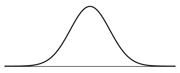
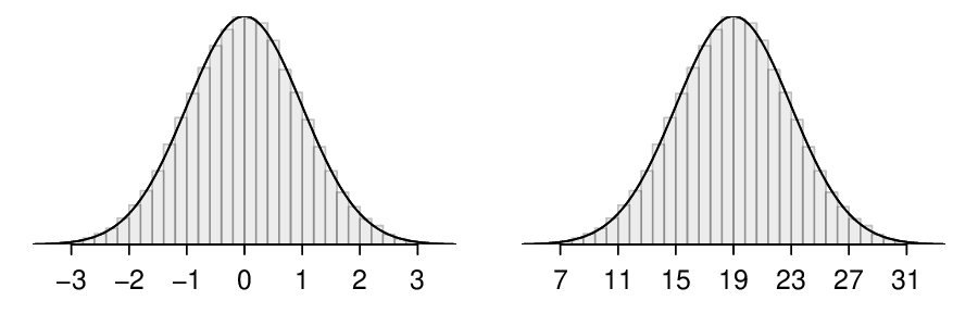
The normal distribution always describes a symmetric, unimodal, bell-shaped curve. However, these curves can look different depending on the details of the model. Specifically, the normal distribution model can be adjusted using two parameters: mean and standard deviation. As you can probably guess, changing the mean shifts the bell curve to the left or right, while changing the standard deviation stretches or constricts the curve. Figure 4.1.2 shows the normal distribution with mean \(0\) and standard deviation \(1\) in the left panel and the normal distributions with mean \(19\) and standard deviation \(4\) in the right panel. Figure 4.1.3 shows these distributions on the same axis.
Because the mean and standard deviation describe a normal distribution exactly, they are called the distribution's parameters. The normal distribution with mean \(\mu=0\) and standard deviation \(\sigma = 1\) is called the standard normal distribution..
Normal distribution facts.
Many variables are nearly normal, but none are exactly normal. The normal distribution, while never perfect, provides very close approximations for a variety of scenarios. We will use it to model data as well as probability distributions.
Subsection 4.1.3 Standardizing with Z-scores
We often want to put data onto a standardized scale, which can make comparisons more reasonable.
Example 4.1.4.
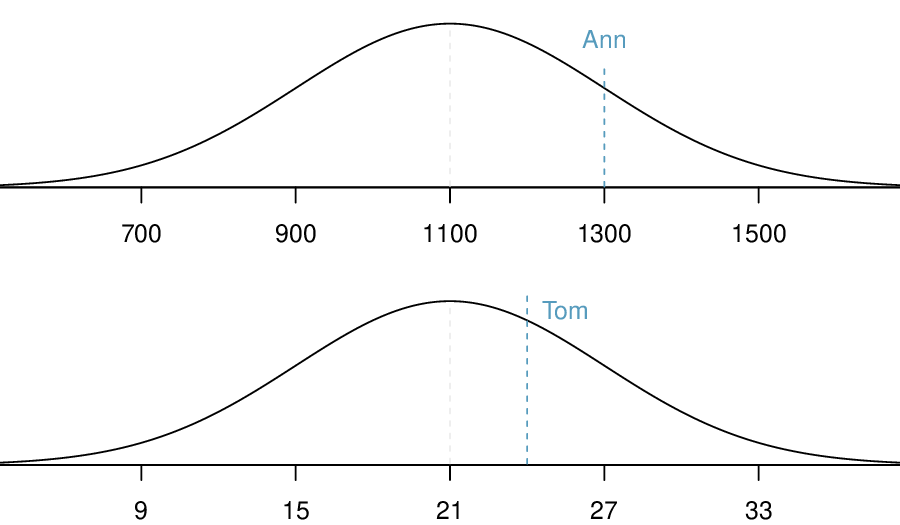
Table 4.1.5 shows the mean and standard deviation for total scores on the SAT and ACT. The distribution of SAT and ACT scores are both nearly normal. Suppose Ann scored 1300 on her SAT and Tom scored 24 on his ACT. Who performed better?
We use the standard deviation as a guide. Ann is 1 standard deviation above average on the SAT: \(1100+200= 1300\text{.}\) Tom is 0.5 standard deviations above the mean on the ACT: \(21 + 0.5 \times 6 = 24\text{.}\) In Figure 4.1.6, we can see that Ann tends to do better with respect to everyone else than Tom did, so her score was better.
| SAT | ACT | |
| Mean | 1100 | 21 |
| SD | 200 | 6 |
Example 4.1.4 used a standardization technique called a Z-score, a method most commonly employed for nearly normal observations but that may be used with any distribution. Recall from Chapter 2 that the Z-score of an observation is defined as the number of standard deviations it falls above or below the mean. If the observation is one standard deviation above the mean, its Z-score is 1. If it is 1.5 standard deviations below the mean, then its Z-score is -1.5. If \(x\) is an observation from a distribution with mean \(\mu\) and standard deviation \(\sigma\text{,}\) we define the Z-score mathematically as
Using \(\mu_{\text{SAT}} = 1100\text{,}\) \(\sigma_{\text{SAT}} = 200\text{,}\) and \(x_{\text{Ann}} = 1300\text{,}\) we find Ann's Z-score:
Checkpoint 4.1.7.
Use Tom's ACT score, 24, along with the ACT mean and standard deviation to find his Z-score. 2
Subsection 4.1.4 Normal probability table
Example 4.1.8.
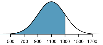
Ann from Example 4.1.4 earned a score of 1300 on her SAT with a corresponding \(Z=1\text{.}\) She would like to know what percentile she falls in among all SAT test-takers.
Ann's percentile is the percentage of people who earned a lower SAT score than Ann. We shade the area representing those individuals in Figure 4.1.9. The total area under the normal curve is always equal to 1, and the proportion of people who scored below Ann on the SAT is equal to the area shaded in Figure 4.1.9: 0.8413. In other words, Ann is in the \(84^{th}\) percentile of SAT takers.
We can use the normal model to find percentiles. A normal probability table, which lists Z-scores and corresponding percentiles, can be used to identify a percentile based on the Z-score (and vice versa). Statistical software can also be used.
A normal probability table is given in Table B.2.1 and abbreviated in Table 4.1.11. We use this table to identify the percentile corresponding to any particular Z-score. For instance, the percentile of \(Z=0.43\) is shown in row \(0.4\) and column \(0.03\) in Table 4.1.11: 0.6664, or the \(66.64^{th}\) percentile. Generally, we round \(Z\) to two decimals, identify the proper row in the normal probability table up through the first decimal, and then determine the column representing the second decimal value. The intersection of this row and column is the percentile of the observation.
| Second decimal place of \(Z\) | ||||||||||
| \(Z\) | 0.00 | 0.01 | 0.02 | 0.03 | 0.04 | 0.05 | 0.06 | 0.07 | 0.08 | 0.09 |
| 0.0 | 0.5000 | 0.5040 | 0.5080 | 0.5120 | 0.5160 | 0.5199 | 0.5239 | 0.5279 | 0.5319 | 0.5359 |
| 0.1 | 0.5398 | 0.5438 | 0.5478 | 0.5517 | 0.5557 | 0.5596 | 0.5636 | 0.5675 | 0.5714 | 0.5753 |
| 0.2 | 0.5793 | 0.5832 | 0.5871 | 0.5910 | 0.5948 | 0.5987 | 0.6026 | 0.6064 | 0.6103 | 0.6141 |
| 0.3 | 0.6179 | 0.6217 | 0.6255 | 0.6293 | 0.6331 | 0.6368 | 0.6406 | 0.6443 | 0.6480 | 0.6517 |
| 0.4 | 0.6554 | 0.6591 | 0.6628 | 0.6664 | 0.6700 | 0.6736 | 0.6772 | 0.6808 | 0.6844 | 0.6879 |
| 0.5 | 0.6915 | 0.6950 | 0.6985 | 0.7019 | 0.7054 | 0.7088 | 0.7123 | 0.7157 | 0.7190 | 0.7224 |
| 0.6 | 0.7257 | 0.7291 | 0.7324 | 0.7357 | 0.7389 | 0.7422 | 0.7454 | 0.7486 | 0.7517 | 0.7549 |
| 0.7 | 0.7580 | 0.7611 | 0.7642 | 0.7673 | 0.7704 | 0.7734 | 0.7764 | 0.7794 | 0.7823 | 0.7852 |
| 0.8 | 0.7881 | 0.7910 | 0.7939 | 0.7967 | 0.7995 | 0.8023 | 0.8051 | 0.8078 | 0.8106 | 0.8133 |
| \(\vdots\) | \(\vdots\) | \(\vdots\) | \(\vdots\) | \(\vdots\) | \(\vdots\) | \(\vdots\) | \(\vdots\) | \(\vdots\) | \(\vdots\) | \(\vdots\) |
We can also find the Z-score associated with a percentile. For example, to identify Z for the \(80^{th}\) percentile, we look for the value closest to 0.8000 in the middle portion of the table: 0.7995. We determine the Z-score for the \(80^{th}\) percentile by combining the row and column Z values: 0.84.
Checkpoint 4.1.12.
Determine the proportion of SAT test takers who scored better than Ann on the SAT. 3
Subsection 4.1.5 Normal probability examples
Cumulative SAT scores are approximated well by a normal model with mean 1100 and standard deviation 200.
Example 4.1.13.
What is the probability that a randomly selected SAT taker scores at least 1190 on the SAT?
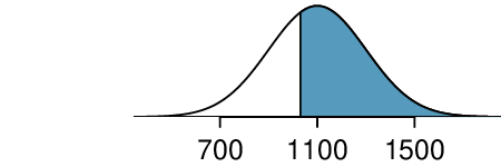
The probability that a randomly selected SAT taker scores at least 1190 on the SAT is equivalent to the proportion of all SAT takers that score at least 1190 on the SAT. First, always draw and label a picture of the normal distribution. (Drawings need not be exact to be useful.) We are interested in the probability that a randomly selected score will be above 1190, so we shade this upper tail:

The picture shows the mean and the values at 2 standard deviations above and below the mean. The simplest way to find the shaded area under the curve makes use of the Z-score of the cutoff value. With \(\mu=1100\text{,}\) \(\sigma=200\text{,}\) and the cutoff value \(x=1190\text{,}\) the Z-score is computed as
We look up the percentile of \(Z=0.45\) in the normal probability table shown in Table 4.1.11 or in Table B.2.1, which yields 0.6736. However, the percentile describes those who had a Z-score lower than 0.45. To find the area above \(Z=0.45\text{,}\) we compute one minus the area of the lower tail:
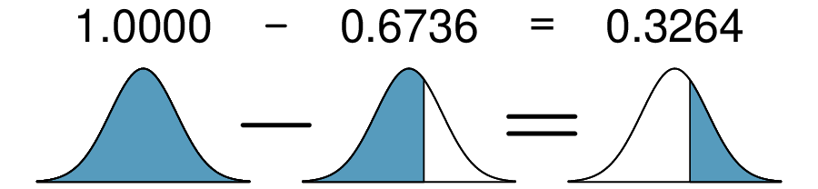
The probability that a randomly selected score is at least 1190 on the SAT is 0.3264.
Always draw a picture first, and find the Z-score second.
For any normal probability situation, always always always draw and label the normal curve and shade the area of interest first. The picture will provide an estimate of the probability.
After drawing a figure to represent the situation, identify the Z-score for the observation of interest.
Checkpoint 4.1.14.
If the probability that a randomly selected score is at least 1190 is 0.3264, what is the probability that the score is less than 1190? Draw the normal curve representing this exercise, shading the lower region instead of the upper one. 4
Example 4.1.15.
Edward earned a 1030 on his SAT. What is his percentile?
First, a picture is needed. Edward's percentile is the proportion of people who do not get as high as a 1030. These are the scores to the left of 1030.
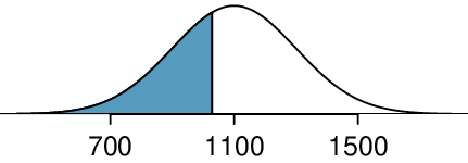
Identifying the mean \(\mu=1100\text{,}\) the standard deviation \(\sigma=200\text{,}\) and the cutoff for the tail area \(x=1030\) makes it easy to compute the Z-score:
Using the normal probability table, identify the row of \(-0.3\) and column of \(0.05\text{,}\) which corresponds to the probability \(0.3632\text{.}\) Edward is at the \(36^{th}\) percentile.
Checkpoint 4.1.16.
Use the results of Example 4.1.15 to compute the proportion of SAT takers who did better than Edward. Also draw a new picture. 5
If Edward did better than 36% of SAT takers, then about 64% must have done better than him.
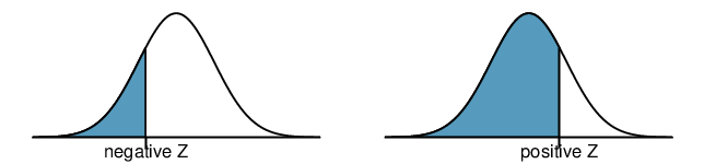
Areas to the right.
The normal probability table in most books gives the area to the left. If you would like the area to the right, first find the area to the left and then subtract this amount from one.
The last several problems have focused on finding the probability or percentile for a particular observation. It is also possible to identify the value corresponding to a particular percentile.
Example 4.1.17.
Carlos believes he can get into his preferred college if he scores at least in the 80th percentile on the SAT. What score should he aim for?
Here, we are given a percentile rather than a Z-score, so we work backwards. As always, first draw the picture.
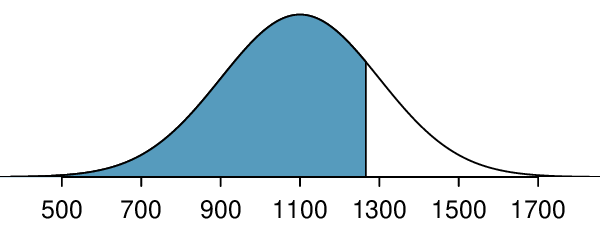
We want to find the observation that corresponds to the 80th percentile. First, we find the Z-score associated with the 80th percentile using the normal probability table. Looking at Table 4.1.11., we look for the number closest to 0.80 inside the table. The closest number we find is 0.7995 (highlighted). 0.7995 falls on row 0.8 and column 0.04, therefore it corresponds to a Z-score of 0.84. In any normal distribution, a value with a Z-score of 0.84 will be at the 80th percentile. Once we have the Z-score, we work backwards to find x.
The 80th percentile on the SAT corresponds to a score of 1268.
Checkpoint 4.1.18.
Imani scored at the 72nd percentile on the SAT. What was her SAT score? 6
If the data are not nearly normal, don't use a normal table.
Before using the normal table, verify that the data or distribution is approximately normal. If it is not, the normal table will give incorrect results. Also, all answers based on normal approximations are approximations and are not exact.
Subsection 4.1.6 Calculator: finding normal probabilities
¶TI-84: Finding area under the normal curve.
Use 2ND VARS, normalcdf to find an area/proportion/probability between two Z-scores or to the left or right of a Z-score.
Choose
2NDVARS(i.e.DISTR).Choose
2:normalcdf.-
Enter the
lower(left) Z-score and theupper(right) Z-score.If finding just a lower tail area, set
lowerto-5.If finding just an upper tail area, set
upperto5.
Leave \(\mu\) as
0and \(\sigma\) as1.Down arrow, choose
Paste, and hitENTER.
TI-83: Do steps 1-2, then enter the lower bound and upper bound separated by a comma, e.g. normalcdf(2, 5), and hit ENTER.
Casio fx-9750GII: Finding area under the normal curve.
Navigate to
STAT(MENU, then hit2).Select
DIST(F5), thenNORM(F1), and thenNcd(F2).If needed, set
DatatoVariable(Varoption, which isF2).-
Enter the
LowerZ-score and theUpperZ-score. Set \(\sigma\) to1and \(\mu\) to0.If finding just a lower tail area, set
Lowerto-5.For an upper tail area, set
Upperto5.
Hit
EXE, which will return the area probability (p) along with the Z-scores for the lower and upper bounds.
Example 4.1.19.
Use a calculator to determine what percentile corresponds to a Z-score of 1.5.
Always first sketch a graph: 7
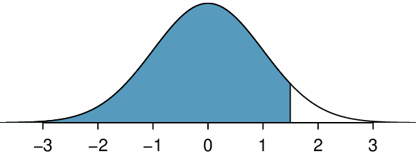
To find an area under the normal curve using a calculator, first identify a lower bound and an upper bound. Theoretically, we want all of the area to the left of 1.5, so the left endpoint should be -\(\infty\text{.}\) However, the area under the curve is nearly negligible when \(Z\) is smaller than -4, so we will use -5 as the lower bound when not given a lower bound (any other negative number smaller than -5 will also work). Using a lower bound of -5 and an upper bound of 1.5, we get \(P(Z \lt 1.5) = 0.933\text{.}\)
Checkpoint 4.1.20.
Find the area under the normal curve to right of \(Z=2\text{.}\) 8
Checkpoint 4.1.21.
Find the area under the normal curve between -1.5 and 1.5. 9
TI-84: Find a Z-score that corresponds to a percentile.
Use 2ND VARS, invNorm to find the Z-score that corresponds to a given percentile.
Choose
2NDVARS(i.e.DISTR).Choose
3:invNorm.Let
Areabe the percentile as a decimal (the area to the left of desired Z-score).Leave \(\mu\) as
0and \(\sigma\) as1.Down arrow, choose
Paste, and hitENTER.
TI-83: Do steps 1-2, then enter the percentile as a decimal, e.g. invNorm(.40)}, then hit ENTER.
Casio fx-9750GII: Find a Z-score that corresponds to a percentile.
Navigate to
STAT(MENU, then hit2).Select
DIST(F5), thenNORM(F1), and thenInvN(F3).If needed, set
DatatoVariable(Varoption, which isF2).Decide which tail area to use (
Tail), the tail area (Area), and then enter the \(\sigma\) and \(\mu\) values.Hit
EXE.
Example 4.1.22.
Use a calculator to find the Z-score that corresponds to the 40th percentile.
Letting Area be 0.40, a calculator gives -0.253. This means that \(Z = -0.253\) corresponds to the 40th percentile, that is, \(P(Z \lt -0.253) = 0.40\text{.}\)
Checkpoint 4.1.23.
Find the Z-score such that 20 percent of the area is to the right of that Z-score. 10
Example 4.1.24.
In a large study of birth weight of newborns, the weights of 23,419 newborn boys were recorded. 11 The distribution of weights was approximately normal with a mean of 7.44 lbs (3376 grams) and a standard deviation of 1.33 lbs (603 grams). The government classifies a newborn as having low birth weight if the weight is less than 5.5 pounds. What percent of these newborns had a low birth weight?
We find an area under the normal curve between -5 (or a number smaller than -5, e.g. -10) and a Z-score that we will calculate. There is no need to write calculator commands in a solution. Instead, continue to use standard statistical notation.
Approximately 6.8% of the newborns were of low birth weight.
Checkpoint 4.1.25.
Approximately what percent of these babies weighed greater than 10 pounds? 12
Checkpoint 4.1.26.
Approximately how many of these newborns weighed greater than 10 pounds? 13
Checkpoint 4.1.27.
How much would a newborn have to weigh in order to be at the 90th percentile among this group? 14
Subsection 4.1.7 68-95-99.7 rule
Here, we present a useful rule of thumb for the probability of falling within 1, 2, and 3 standard deviations of the mean in the normal distribution. This will be useful in a wide range of practical settings, especially when trying to make a quick estimate without a calculator or Z table.

Checkpoint 4.1.29.
Use the Z table to confirm that about 68%, 95%, and 99.7% of observations fall within 1, 2, and 3, standard deviations of the mean in the normal distribution, respectively. For instance, first find the area that falls between \(Z=-1\) and \(Z=1\text{,}\) which should have an area of about 0.68. Similarly there should be an area of about 0.95 between \(Z=-2\) and \(Z=2\text{.}\) 15
It is possible for a normal random variable to fall 4, 5, or even more standard deviations from the mean. However, these occurrences are very rare if the data are nearly normal. The probability of being further than 4 standard deviations from the mean is about 1-in-15,000. For 5 and 6 standard deviations, it is about 1-in-2 million and 1-in-500 million, respectively.
Checkpoint 4.1.30.
SAT scores closely follow the normal model with mean \(\mu = 1100\) and standard deviation \(\sigma = 200\text{.}\) (a) About what percent of test takers score 700 to 1500? (b) What percent score between 1100 and 1500? 16
Subsection 4.1.8 Evaluating the normal approximation
¶It is important to remember normality is always an approximation. Testing the appropriateness of the normal assumption is a key step in many data analyses.
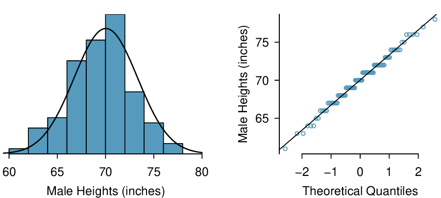
The distribution of heights of US males is well approximated by the normal model. We are interested in proceeding under the assumption that the data are normally distributed, but first we must check to see if this is reasonable.
There are two visual methods for checking the assumption of normality that can be implemented and interpreted quickly. The first is a simple histogram with the best fitting normal curve overlaid on the plot, as shown in the left panel of Figure 4.1.31. The sample mean \(\bar{x}\) and standard deviation \(s\) are used as the parameters of the best fitting normal curve. The closer this curve fits the histogram, the more reasonable the normal model assumption. Another more common method is examining a normal probability plot, 17 shown in the right panel of Figure 4.1.31. The closer the points are to a perfect straight line, the more confident we can be that the data follow the normal model.
Three data sets of 40, 100, and 400 samples were simulated from a normal distribution, and the histograms and normal probability plots of the data sets are shown in Figure 4.1.32. These will provide a benchmark for what to look for in plots of real data.

The left panels show the histogram (top) and normal probability plot (bottom) for the simulated data set with 40 observations. The data set is too small to really see clear structure in the histogram. The normal probability plot also reflects this, where there are some deviations from the line. However, these deviations are not strong.
The middle panels show diagnostic plots for the data set with 100 simulated observations. The histogram shows more normality and the normal probability plot shows a better fit. While there is one observation that deviates noticeably from the line, it is not particularly extreme.
The data set with 400 observations has a histogram that greatly resembles the normal distribution, while the normal probability plot is nearly a perfect straight line. Again in the normal probability plot there is one observation (the largest) that deviates slightly from the line. If that observation had deviated 3 times further from the line, it would be of much greater concern in a real data set. Apparent outliers can occur in normally distributed data but they are rare.
Notice the histograms look more normal as the sample size increases, and the normal probability plot becomes straighter and more stable.
Example 4.1.33.
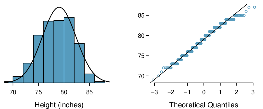
Consider all NBA players from the 2018-2019 season presented in Figure 4.1.34. 18 Based on the graphs, are NBA player heights normally distributed?
We first create a histogram and normal probability plot of the NBA player heights. The histogram in the left panel is slightly left skewed, which contrasts with the symmetric normal distribution. The points in the normal probability plot do not appear to closely follow a straight line but show what appears to be a “wave”. We can compare these characteristics to the sample of 400 normally distributed observations in Figure 4.1.32 and see that they represent much stronger deviations from the normal model. NBA player heights do not appear to come from a normal distribution.
Example 4.1.35.
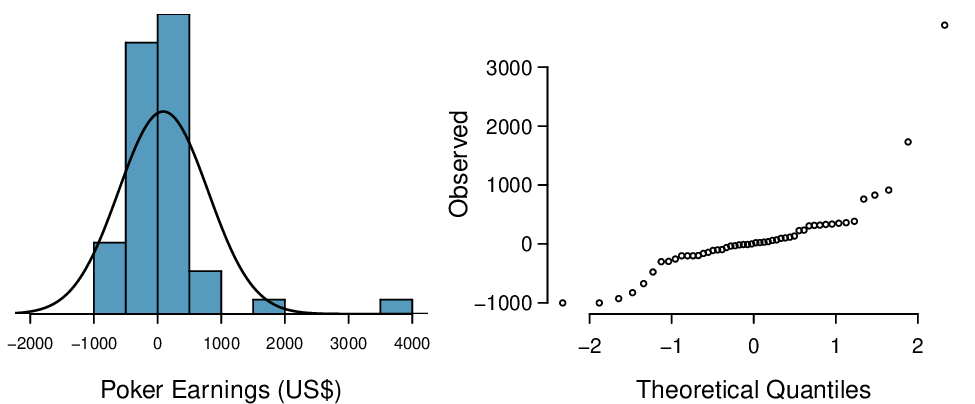
Consider the poker winnings of an individual over 50 days. A histogram and normal probability plot of these data are shown in Figure 4.1.36. Based on the graphs, can we approximate poker winnings by a normal distribution?
The data are very strongly right skewed in the histogram, which corresponds to the very strong deviations on the upper right component of the normal probability plot. If we compare these results to the sample of 40 normal observations in Figure 4.1.32, it is apparent that these data show very strong deviations from the normal model.
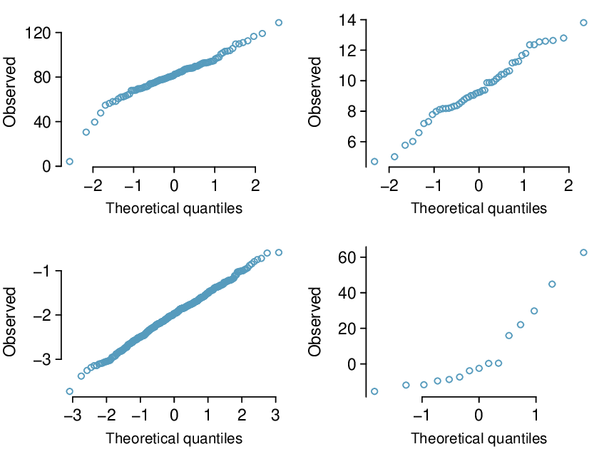
Checkpoint 4.1.37.
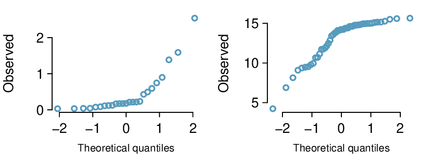
Determine which data sets represented in Figure 4.1.38 plausibly come from a nearly normal distribution. Are you confident in all of your conclusions? There are 100 (top left), 50 (top right), 500 (bottom left), and 15 points (bottom right) in the four plots. 19
Checkpoint 4.1.39.
Figure 4.1.40 shows normal probability plots for two distributions that are skewed. One distribution is skewed to the low end (left skewed) and the other to the high end (right skewed). Which is which? 20
Subsection 4.1.9 Normal approximation for sums of random variables
¶We have seen that many distributions are approximately normal. The sum and the difference of normally distributed variables is also normal. While we cannot prove this here, the usefulness of it is seen in the following example.
Example 4.1.41.
Three friends are playing a cooperative video game in which they have to complete a puzzle as fast as possible. Assume that the individual times of the 3 friends are independent of each other. The individual times of the friends in similar puzzles are approximately normally distributed with the following means and standard deviations.
| Mean | SD | |
| Friend 1 | 5.6 | 0.11 |
| Friend 2 | 5.8 | 0.13 |
| Friend 3 | 6.1 | 0.12 |
To advance to the next level of the game, the friends' total time must not exceed 17.1 minutes. What is the probability that they will advance to the next level?
Because each friend's time is approximately normally distributed, the sum of their times is also approximately normally distributed. We will do a normal approximation, but first we need to find the mean and standard deviation of the sum. We learned how to do this in Section 3.5.
Let the three friends be labeled \(X\text{,}\) \(Y\text{,}\) \(Z\text{.}\) We want \(P(X + Y + Z \lt 17.1)\text{.}\) The mean and standard deviation of the sum of \(X\text{,}\) \(Y\text{,}\) and \(Z\) is given by:
Now we can find the Z-score.
Finally, we want the probability that the sum is less than 17.5, so we shade the area to the left of \(Z = -1.92\text{.}\) Using the normal table or a calculator, we get
There is a 2.7% chance that the friends will advance to the next level.
Checkpoint 4.1.42.
What is the probability that Friend 2 will complete the puzzle with a faster time than Friend 1? Hint: find \(P(Y \lt X)\text{,}\) or \(P(Y - X \lt 0)\text{.}\) 21
Subsection 4.1.10 Section summary
A Z-score represents the number of standard deviations a value in a data set is above or below the mean. To calculate a \(Z\)-score use: \(Z = \frac{x-\text{ mean } }{SD}\text{.}\)
Z-scores do not depend on units. When looking at distributions with different units or different standard deviations, \(Z\)-scores are useful for comparing how far values are away from the mean (relative to the distribution of the data).
The normal distribution is the most commonly used distribution in Statistics. Many distribution are approximately normal, but none are exactly normal.
The empirical rule (68-95-99.7 Rule) comes from the normal distribution. The closer a distribution is to normal, the better this rule will hold.
-
It is often useful to use the standard normal distribution, which has mean 0 and SD 1, to approximate a discrete histogram. There are two common types of normal approximation problems, and for each a key step is to find a \(Z\)-score.
-
Find the percent or probability of a value greater/less than a given \(x\)-value.
Verify that the distribution of interest is approximately normal.
Calculate the \(Z\)-score . Use the provided population mean and SD to standardize the given \(x\)-value.
Use a calculator function (e.g.
normcdfon a TI) or a normal table to find the area under the normal curve to the right/left of this \(Z\)-score ; this is the estimate for the percent/probability.
-
Find the x-value that corresponds to a given percentile.
Verify that the distribution of interest is approximately normal.
Find the \(Z\)-score that corresponds to the given percentile (using, for example,
invNormon a TI).Use the \(Z\)-score along with the given mean and SD to solve for the x-value.
-
Because the sum or difference of two normally distributed variables is itself a normally distributed variable, the normal approximation is also used in the following type of problem.
-
Find the probability that a sum \(X+Y\) or a difference \(X-Y\) is greater/less than some value.
Verify that the distribution of \(X\) and the distribution of \(Y\) are approximately normal.
Find the mean of the sum or difference. Recall: the mean of a sum is the sum of the means. The mean of a difference is the difference of the means. Find the SD of the sum or difference using: \(SD(X+Y) = SD(X - Y) = \sqrt{(SD(X))^2 + (SD(Y))^2}\text{.}\)
Calculate the \(Z\)-score. Use the calculated mean and SD to standardize the given sum or difference.
Find the appropriate area under the normal curve.
Exercises 4.1.11 Exercises
1. Area under the curve, Part I.
What percent of a standard normal distribution \(N(\mu=0, \sigma=1)\) is found in each region? Be sure to draw a graph.
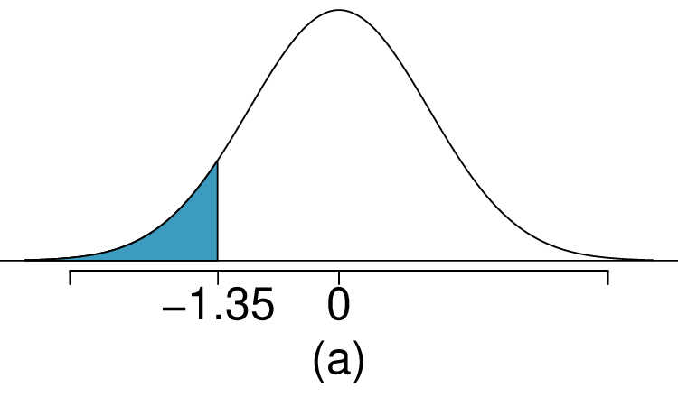
\(Z \lt -1.35\)
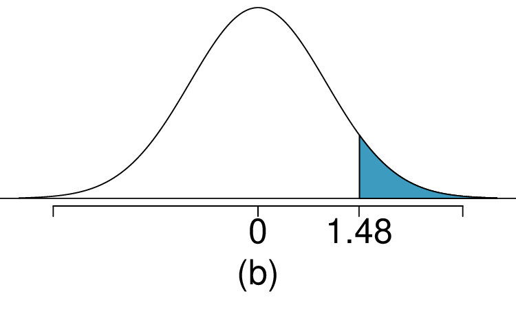
\(Z > 1.48\)
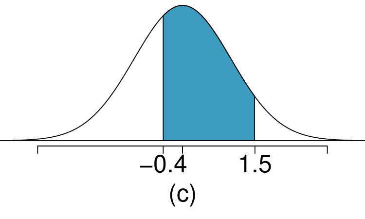
\(-0.4 \lt Z \lt 1.5\)
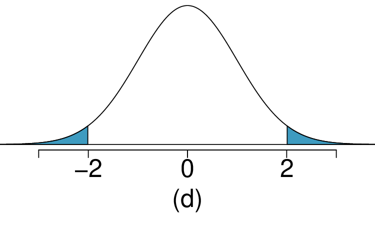
\(|Z| > 2\)
(a) 8.85%. (b) 6.94%. (c) 58.86%. (d) 4.56%.
2. Area under the curve, Part II.
What percent of a standard normal distribution \(N(\mu=0, \sigma=1)\) is found in each region? Be sure to draw a graph.
\(Z > -1.13\)
\(Z \lt 0.18\)
\(Z > 8\)
\(|Z| \lt 0.5\)
3. GRE scores, Part I.
Sophia who took the Graduate Record Examination (GRE) scored 160 on the Verbal Reasoning section and 157 on the Quantitative Reasoning section. The mean score for Verbal Reasoning section for all test takers was 151 with a standard deviation of 7, and the mean score for the Quantitative Reasoning was 153 with a standard deviation of 7.67. Suppose that both distributions are nearly normal.
What is Sophia's Z-score on the Verbal Reasoning section? On the Quantitative Reasoning section? Draw a standard normal distribution curve and mark these two Z-scores.
What do these Z-scores tell you?
Relative to others, which section did she do better on?
Find her percentile scores for the two exams.
What percent of the test takers did better than her on the Verbal Reasoning section? On the Quantitative Reasoning section?
Explain why simply comparing raw scores from the two sections could lead to an incorrect conclusion as to which section a student did better on.
If the distributions of the scores on these exams are not nearly normal, would your answers to parts (b) - (e) change? Explain your reasoning.
(a) \(Z_{VR} = 1.29\text{,}\) \(Z_{QR} = 0.52\text{.}\)
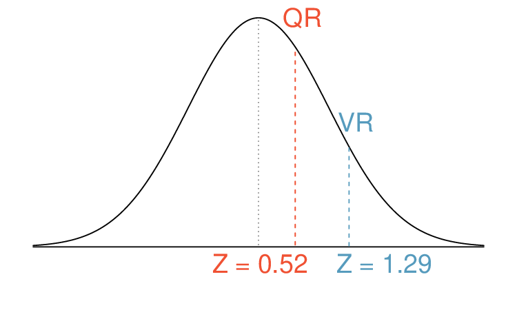
(b) She scored 1.29 standard deviations above the mean on the Verbal Reasoning section and 0.52 standard deviations above the mean on the Quantitative Reasoning section.
(c) She did better on the Verbal Reasoning section since her Z-score on that section was higher.
(d) \(\text{Percentile}_{VR} = 0.9007 \approx 90%\text{,}\) \(\text{Percentile}_{QR} = 0.6990 \approx 70%\text{.}\)
(e) \(100%-90% = 10%\) did better than her on VR, and \(100% - 70% = 30%\) did better than her on QR.
(f) We cannot compare the raw scores since they are on different scales. Comparing her percentile scores is more appropriate when comparing her performance to others.
(g) Answer to part (b) would not change as Z-scores can be calculated for distributions that are not normal. However, we could not answer parts (c)-(e) since we cannot use the normal probability table to calculate probabilitiesand percentiles without a normal model.
4. Triathlon times, Part I.
In triathlons, it is common for racers to be placed into age and gender groups. Friends Leo and Mary both completed the Hermosa Beach Triathlon, where Leo competed in the Men, Ages 30 - 34 group while Mary competed in the Women, Ages 25 - 29 group. Leo completed the race in 1:22:28 (4948 seconds), while Mary completed the race in 1:31:53 (5513 seconds). Obviously Leo finished faster, but they are curious about how they did within their respective groups. Can you help them? Here is some information on the performance of their groups:
The finishing times of the Men, Ages 30 - 34 group has a mean of 4313 seconds with a standard deviation of 583 seconds.
The finishing times of the Women, Ages 25 - 29 group has a mean of 5261 seconds with a standard deviation of 807 seconds.
The distributions of finishing times for both groups are approximately Normal.
Remember: a better performance corresponds to a faster finish.
What are the Z-scores for Leo's and Mary's finishing times? What do these Z-scores tell you?
Did Leo or Mary rank better in their respective groups? Explain your reasoning.
What percent of the triathletes did Leo finish faster than in his group?
What percent of the triathletes did Mary finish faster than in her group?
If the distributions of finishing times are not nearly normal, would your answers to parts (a) - (d) change? Explain your reasoning.
5. GRE scores, Part II.
In Exercise 4.1.11.3 we saw two distributions for GRE scores: \(N(\mu=151, \sigma=7)\) for the verbal part of the exam and \(N(\mu=153, \sigma=7.67)\) for the quantitative part. Use this information to compute each of the following:
The score of a student who scored in the \(80^{th}\) percentile on the Quantitative Reasoning section.
The score of a student who scored worse than 70% of the test takers in the Verbal Reasoning section.
(a) \(Z = 0.84\text{,}\) which corresponds to approximately 160 on QR.
(b) \(Z = -0.52\text{,}\) which corresponds to approximately 147 on VR.
6. Triathlon times, Part II.
In Exercise 4.1.11.4 we saw two distributions for triathlon times: \(N(\mu=4313, \sigma=583)\) for Men, Ages 30 - 34 and \(N(\mu=5261, \sigma=807)\) for the Women, Ages 25 - 29 group. Times are listed in seconds. Use this information to compute each of the following:
The cutoff time for the fastest 5% of athletes in the men's group, i.e. those who took the shortest 5% of time to finish.
The cutoff time for the slowest 10% of athletes in the women's group.
7. LA weather, Part I.
The average daily high temperature in June in LA is 77°F with a standard deviation of 5°F. Suppose that the temperatures in June closely follow a normal distribution.
What is the probability of observing an 83°F temperature or higher in LA during a randomly chosen day in June?
How cool are the coldest 10% of the days (days with lowest average high temperature) during June in LA?
(a) \(Z = 1.2 \rightarrow 0.1151\text{.}\)
(b) \(Z = -1.28 \rightarrow 70.6\)°F or colder.
8. CAPM.
The Capital Asset Pricing Model (CAPM) is a financial model that assumes returns on a portfolio are normally distributed. Suppose a portfolio has an average annual return of 14.7% (i.e. an average gain of 14.7%) with a standard deviation of 33%. A return of 0% means the value of the portfolio doesn't change, a negative return means that the portfolio loses money, and a positive return means that the portfolio gains money.
What percent of years does this portfolio lose money, i.e. have a return less than 0%?
What is the cutoff for the highest 15% of annual returns with this portfolio?
9. LA weather, Part II.
Exercise 4.1.11.7 states that average daily high temperature in June in LA is 77°F with a standard deviation of 5°F, and it can be assumed that they to follow a normal distribution. We use the following equation to convert °F (Fahrenheit) to °C (Celsius):
What is the probability of observing a 28°C (which roughly corresponds to 83°F) temperature or higher in June in LA? Calculate using the °C model from part (a).
Did you get the same answer or different answers in part (b) of this question and part (a) of Exercise 4.1.11.7? Are you surprised? Explain.
Estimate the IQR of the temperatures (in °C) in June in LA.
(a) \(Z = 1.08 \rightarrow 0.1401\text{.}\)
(b) The answers are very close because only the units were changed. (The only reason why they are a little different is because 28°C is 82.4°F, not precisely 83°F.)
(c) Since \(IQR = Q3 - Q1\text{,}\) we first need to find Q3 and Q1 and take the difference between the two. Remember that Q3 is the 75th and Q1 is the 25th Percentile of a distribution. \(Q1 = 23.13\text{,}\) \(Q3 = 26.86\text{,}\) \(IQR = 26.86 - 23.13 = 3.73\text{.}\)
10. Find the SD.
Cholesterol levels for women aged 20 to 34 follow an approximately normal distribution with mean 185 milligrams per deciliter (mg/dl). Women with cholesterol levels above 220 mg/dl are considered to have high cholesterol and about 18.5% of women fall into this category. Find the standard deviation of this distribution.
11. Scores on stats final, Part I.
Below are final exam scores of 20 Introductory Statistics students.
The mean score is 77.7 points. with a standard deviation of 8.44 points. Use this information to determine if the scores approximately follow the 68-95-99.7% Rule.
\(14/20 = 70%\) are within 1 SD. Within 2 SD: \(19/20 = 95%\text{.}\) Within 3 SD: \(20/20 = 100%\text{.}\) They follow this rule closely.
12. Heights of female college students, Part I.
Below are heights of 25 female college students.
The mean height is 61.52 inches with a standard deviation of 4.58 inches. Use this information to determine if the heights approximately follow the 68-95-99.7% Rule.
13. Lemonade at The Cafe.
Drink pitchers at The Cafe are intended to hold about 64 ounces of lemonade and glasses hold about 12 ounces. However, when the pitchers are filled by a server, they do not always fill it with exactly 64 ounces. There is some variability. Similarly, when they pour out some of the lemonade, they do not pour exactly 12 ounces. The amount of lemonade in a pitcher is normally distributed with mean 64 ounces and standard deviation 1.732 ounces. The amount of lemonade in a glass is normally distributed with mean 12 ounces and standard deviation 1 ounce.
How much lemonade would you expect to be left in a pitcher after pouring one glass of lemonade?
What is the standard deviation of the amount left in a pitcher after pouring one glass of lemonade?
What is the probability that more than 50 ounces of lemonade is left in a pitcher after pouring one glass of lemonade?
(a) Let X represent the amount of lemonade in the pitcher, Y represent the amount of lemonade in a glass, and W represent the amount left over after. Then, \(\mu_{W} = E(X - Y ) = 64 - 12 = 52\)
(b) \(\sigma_{W} = \sqrt{SD(X)^2 + SD(Y)^2} = \sqrt{1.732^2 + 1^2} \approx \sqrt{4} = 2\)
(c) \(P(W > 50) = P(Z > \frac{50-52}{2})= P(Z > -1) = 1 - 0.1587 = 0.8413\)
14. Spray paint, Part I.
Suppose the area that can be painted using a single can of spray paint is slightly variable and follows a nearly normal distribution with a mean of 25 square feet and a standard deviation of 3 square feet. Suppose also that you buy three cans of spray paint.
How much area would you expect to cover with these three cans of spray paint?
What is the standard deviation of the area you expect to cover with these three cans of spray paint?
The area you wanted to cover is 80 square feet. What is the probability that you will be able to cover this entire area with these three cans of spray paint?
15. GRE scores, Part III.
In Exercise 4.1.11.3 and Exercise 4.1.11.5 we saw two distributions for GRE scores: \(N(\mu=151, \sigma=7)\) for the verbal part of the exam and \(N(\mu=153, \sigma=7.67)\) for the quantitative part. Suppose performance on these two sections is independent. Use this information to compute each of the following:
The probability of a combined (verbal + quantitative) score above 320.
The score of a student who scored better than 90% of the test takers overall.
(a) The combined scores follow a normal distribution with \(\mu_{\text{combined}}= 304\) and \(\sigma_{\text{combined}}= 10.38\text{.}\) Then, \(P(\text{combined score} > 320)\) is approximately 0.06.
(b) \(Z=1.28\) (using calculator or table). Then we set \(1.28 = \frac{x-304}{10.38}\) and find \(x \approx 317\text{.}\)
16. Betting on dinner, Part I.
Suppose a restaurant is running a promotion where prices of menu items are random following some underlying distribution. If you're lucky, you can get a basket of fries for $3, or if you're not so lucky you might end up having to pay $10 for the same menu item. The price of basket of fries is drawn from a normal distribution with mean $6 and standard deviation of $2. The price of a fountain drink is drawn from a normal distribution with mean $3 and standard deviation of $1. What is the probability that you pay more than $10 for a dinner consisting of a basket of fries and a fountain drink?