Section 3.6 Continuous distributions
¶So far we have looked only at cases where the random variable takes on integer values. What happens when we consider random variables that produce a continuous numerical variable, such as wait time for a bus? In this section, we introduce the concept of a continuous distribution. In the next chapter, you will encounter the most famous continuous distribution of all. 1
Subsection 3.6.1 Learning objectives
Understand the difference between a discrete random variable and a continuous random variable.
Recognize that when working with continuous probability distributions area represents probability and the total area under the curve must equal 1.
Subsection 3.6.2 From histograms to continuous distributions
Example 3.6.1.
Figure 3.6.2 shows a few different hollow histograms of the variable height for 3 million US adults from the mid-90's. How does changing the number of bins allow you to make different interpretations of the data?
Adding more bins provides greater detail. This sample is extremely large, which is why much smaller bins still work well. Usually we do not use so many bins with smaller sample sizes since small counts per bin mean the bin heights are very volatile.
Example 3.6.3.
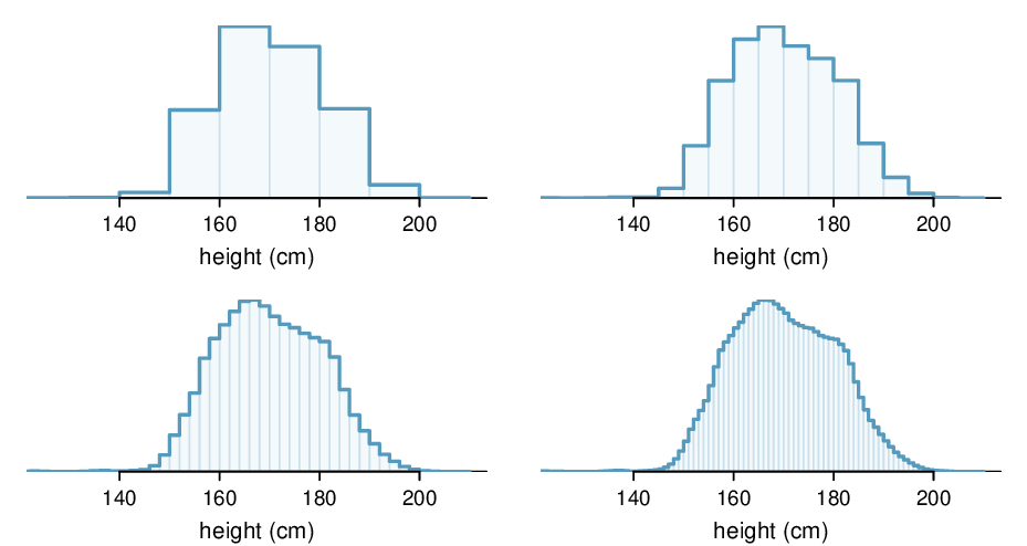
What proportion of the sample is between 180 cm and 185 cm tall (about 5'11" to 6'1")?
We can add up the heights of the bins in the range 180 cm and 185 and divide by the sample size. For instance, this can be done with the two shaded bins shown in Figure 3.6.4. The two bins in this region have counts of 195,307 and 156,239 people, resulting in the following estimate of the probability:
This fraction is the same as the proportion of the histogram's area that falls in the range 180 to 185 cm.
Examine the transition from a boxy hollow histogram in the top-left of Figure 3.6.2 to the much smoother plot in the lower-right. In this last plot, the bins are so slim that the hollow histogram is starting to resemble a smooth curve. This suggests the population height as a continuous numerical variable might best be explained by a curve that represents the outline of extremely slim bins.
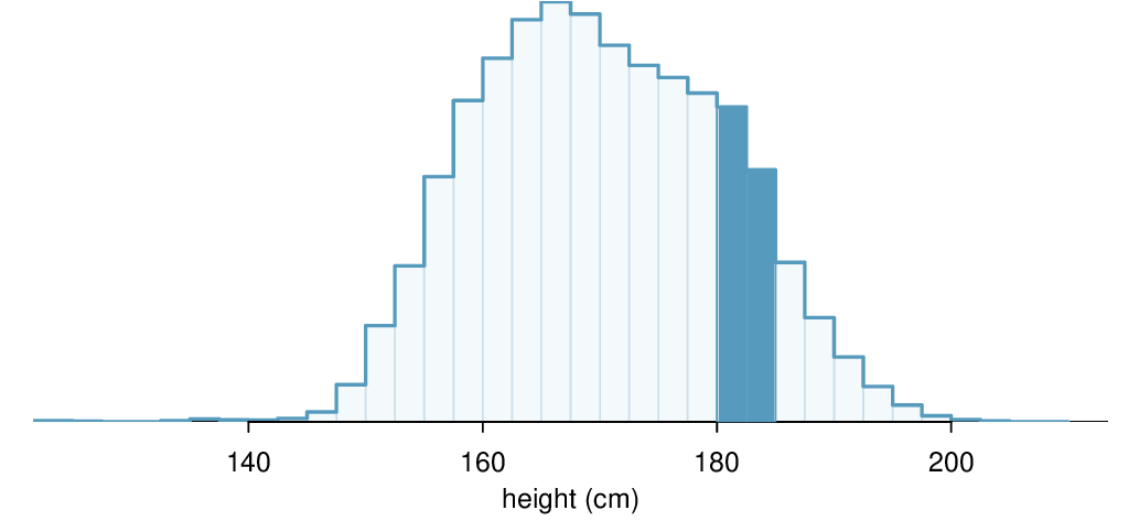
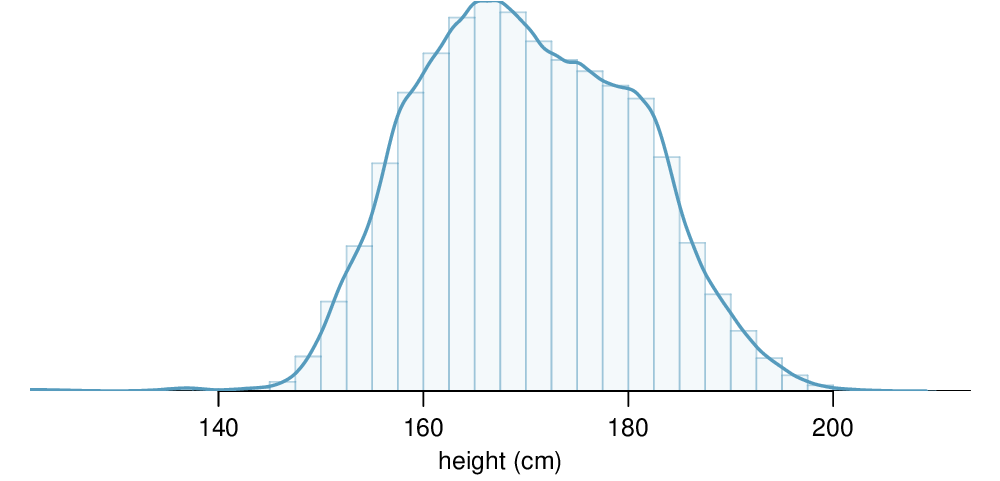
This smooth curve represents a probability density function (also called a density or distribution), and such a curve is shown in Figure 3.6.5 overlaid on a histogram of the sample. A density has a special property: the total area under the density's curve is 1.
Subsection 3.6.3 Probabilities from continuous distributions
We computed the proportion of individuals with heights 180 to 185 cm in Solution 3.6.3.1 as a fraction:
We found the number of people with heights between 180 and 185 cm by determining the fraction of the histogram's area in this region. Similarly, we can use the area in the shaded region under the curve to find a probability (with the help of a computer):
The probability that a randomly selected person is between 180 and 185 cm is 0.1157. This is very close to the estimate from Solution 3.6.3.1: 0.1172.
Checkpoint 3.6.6.
Three US adults are randomly selected. The probability a single adult is between 180 and 185 cm is 0.1157.
What is the probability that all three are between 180 and 185 cm tall?
What is the probability that none are between 180 and 185 cm? 2
Example 3.6.7.
What is the probability that a randomly selected person is exactly 180 cm? Assume you can measure perfectly.
This probability is zero. A person might be close to 180 cm, but not exactly 180 cm tall. This also makes sense with the definition of probability as area; there is no area captured between 180 cm and 180 cm.
Checkpoint 3.6.8.
Suppose a person's height is rounded to the nearest centimeter. Is there a chance that a random person's measured height will be 180 cm? 3
Subsection 3.6.4 Section summary
Histograms use bins with a specific width to display the distribution of a variable. When there is enough data and the data does not have gaps, as the bin width gets smaller and smaller, the histogram begins to resemble a smooth curve, or a continuous distribution.
Continuous distributions are often used to approximate relative frequencies and probabilities. In a continuous distribution, the area under the curve corresponds to relative frequency or probability. The total area under a continuous probability distribution must equal 1.
Because the area under the curve for a single point is zero, the probability of any specific value is zero. This implies that, for example, \(P(X \lt 5) = P(X \le 5)\) for a continuous probability distribution.
Finding areas under curves is challenging; it is common to use distribution tables, calculators, or other technology to find such areas.
Exercises 3.6.5 Exercises
1. Cat weights.
The histogram shown below represents the weights (in kg) of 47 female and 97 male cats. 4
What fraction of these cats weigh less than 2.5 kg?
What fraction of these cats weigh between 2.5 and 2.75 kg?
What fraction of these cats weigh between 2.75 and 3.5 kg?

Approximate answers are OK.
(a) \((29 + 32)/144 = 0.42\text{.}\)
(b) \(21/144 = 0.15\text{.}\)
(c) \((26 + 12 + 15)/144 = 0.37\text{.}\)
2. Income and gender.
The relative frequency table below displays the distribution of annual total personal income (in 2009 inflation-adjusted dollars) for a representative sample of 96,420,486 Americans. These data come from the American Community Survey for 2005-2009. This sample is comprised of 59% males and 41% females. 5
Describe the distribution of total personal income.
What is the probability that a randomly chosen US resident makes less than $50,000 per year?
What is the probability that a randomly chosen US resident makes less than $50,000 per year and is female? Note any assumptions you make.
The same data source indicates that 71.8% of females make less than $50,000 per year. Use this value to determine whether or not the assumption you made in part (c) is valid.
| Income | Total |
| $1 to $9,999 or loss | 2.2% |
| $10,000 to $14,999 | 4.7% |
| $15,000 to $24,999 | 15.8% |
| $25,000 to $34,999 | 18.3% |
| $35,000 to $49,999 | 21.2% |
| $50,000 to $64,999 | 13.9% |
| $65,000 to $74,999 | 5.8% |
| $75,000 to $99,999 | 8.4% |
| $100,000 or more | 9.7% |
Subsection 3.6.6 Chapter Highlights
This chapter focused on understanding likelihood and chance variation, first by solving individual probability questions and then by investigating probability distributions.
The main probability techniques covered in this chapter are as follows:
The General Multiplication Rule for and probabilities (intersection), along with the special case when events are independent.
The General Addition Rule for or probabilities (union), along with the special case when events are mutually exclusive.
The Conditional Probability Rule.
Tree diagrams and Bayes' Theorem to solve more complex conditional problems.
The Binomial Formula for finding the probability of exactly \(x\) successes in \(n\) independent trials.
Simulations and the use of random digits to estimate probabilities.
Fundamental to all of these problems is understanding when events are independent and when they are mutually exclusive. Two events are independent when the outcome of one does not affect the outcome of the other, i.e. \(P(A | B) = P(A)\text{.}\) Two events are mutually exclusive when they cannot both happen together, i.e. \(P(A \text{ and } B) = 0\text{.}\)
Moving from solving individual probability questions to studying probability distributions helps us better understand chance processes and quantify expected chance variation.
For a discrete probability distribution, the sum of the probabilities must equal 1. For a continuous probability distribution, the area under the curve represents a probability and the total area under the curve must equal 1.
As with any distribution, one can calculate the mean and standard deviation of a probability distribution. In the context of a probability distribution, the mean and standard deviation describe the average and the typical deviation from the average, respectively, after many, many repetitions of the chance process.
A probability distribution can be summarized by its center (mean, median), spread (SD, IQR), and shape (right skewed, left skewed, approximately symmetric).
Adding a constant to every value in a probability distribution adds that value to the mean, but it does not affect the standard deviation. When multiplying every value by a constant, this multiplies the mean by the constant and it multiplies the standard deviation by the absolute value of the constant.
The mean of the sum of two random variables equals the sum of the means. However, this is not true for standard deviations. Instead, when finding the standard deviation of a sum or difference of random variables, take the square root of the sum of each of the standard deviations squared.
The study of probability is useful for measuring uncertainty and assessing risk. In addition, probability serves as the foundation for inference, providing a framework for evaluating when an outcome falls outside of the range of what would be expected by chance alone.