Section 3.2 Conditional probability
¶In this section we will use conditional probabilities to answer the following questions:
What is the likelihood that a machine learning algorithm will misclassify a photo as being about fashion if it is not actually about fashion?
How much more likely are children to attend college whose parents attended college than children whose parents did not attend college?
Given that a person receives a positive test result for a disease, what is the probability that the person actually has the disease?
Subsection 3.2.1 Learning objectives
Understand conditional probability and how to calculate it.
Calculate joint and conditional probabilities based on a two-way table.
Use the General Multiplication Rule to find the probability of joint events.
Determine whether two events are independent and whether they are mutually exclusive, based on the definitions of those terms.
Draw a tree diagram with at least two branches to organize possible outcomes and their probabilities. Understand that the second branch represents conditional probabilities.
Use the tree diagram or Bayes' Theorem to solve “inverted” conditional probabilities.
Subsection 3.2.2 Exploring probabilities with a contingency table
The photo_classify data set represents a sample of 1822 photos from a photo sharing website. Data scientists have been working to improve a classifier for whether the photo is about fashion or not, and these 659 photos represent a test for their classifier. Each photo gets two classifications: the first is called mach_learn and gives a classification from a machine learning (ML) system of either pred_fashion or pred_not. Each of these 1822 photos have also been classified carefully by a team of people, which we take to be the source of truth; this variable is called truth and takes values fashion and not. Table 3.2.1 summarizes the results.
truth |
||||
fashion |
not |
Total | ||
mach_learn |
pred_fashion |
197 | 22 | 219 |
pred_not |
112 | 1491 | 1603 | |
| Total | 309 | 1513 | 1822 | |
photo_classify data set.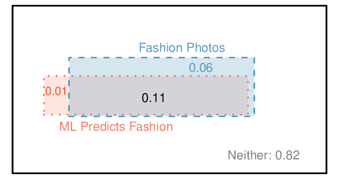
photo_classify data set.Example 3.2.3.
If a photo is actually about fashion, what is the chance the ML classifier correctly identified the photo as being about fashion?
We can estimate this probability using the data. Of the 309 fashion photos, the ML algorithm correctly classified 197 of the photos:
Example 3.2.4.
We sample a photo from the data set and learn the ML algorithm predicted this photo was not about fashion. What is the probability that it was incorrect and the photo is about fashion?
If the ML classifier suggests a photo is not about fashion, then it comes from the second row in the data set. Of these 1603 photos, 112 were actually about fashion:
Subsection 3.2.3 Marginal and joint probabilities
¶Table 3.2.1 includes row and column totals for each variable separately in the photo_classify data set. These totals represent marginal probabilities for the sample, which are the probabilities based on a single variable without regard to any other variables. For instance, a probability based solely on the mach_learn variable is a marginal probability:
A probability of outcomes for two or more variables or processes is called a joint probability:
It is common to substitute a comma for “and” in a joint probability, although using either the word “and” or a comma is acceptable:
Marginal and joint probabilities.
If a probability is based on a single variable, it is a marginal probability . The probability of outcomes for two or more variables or processes is called a joint probability .
We use table proportions to summarize joint probabilities for the photo_classify sample. These proportions are computed by dividing each count in Table 3.2.1 by the table's total, 1822, to obtain the proportions in Table 3.2.5. The joint probability distribution of the mach_learn and truth variables is shown in Table 3.2.6.
truth: fashion
|
truth: not
|
Total | |
mach_learn: pred_fashion
|
0.1081 | 0.0121 | 0.1202 |
mach_learn: pred_not
|
0.0615 | 0.8183 | 0.8798 |
| Total | 0.1696 | 0.8304 | 1.00 |
photo_classify data set.| Joint outcome | Probability |
mach_learn is pred_fashion and truth is fashion
|
0.1081 |
mach_learn is pred_fashion and truth is not
|
0.0121 |
mach_learn is pred_not and truth is fashion
|
0.0615 |
mach_learn is pred_not and truth is not
|
0.8183 |
| Total | 1.0000 |
photo_classify data set.Checkpoint 3.2.7.
Verify Table 3.2.6 represents a probability distribution: events are disjoint, all probabilities are non-negative, and the probabilities sum to 1. 1
We can compute marginal probabilities using joint probabilities in simple cases. For example, the probability that a randomly selected photo from the data set is about fashion is found by summing the outcomes in which truth takes value fashion:
Subsection 3.2.4 Defining conditional probability
The ML classifier predicts whether a photo is about fashion, even if it is not perfect. We would like to better understand how to use information from a variable like mach_learn to improve our probability estimation of a second variable, which in this example is truth.
The probability that a random photo from the data set is about fashion is about 0.17. If we knew the machine learning classifier predicted the photo was about fashion, could we get a better estimate of the probability the photo is actually about fashion? Absolutely. To do so, we limit our view to only those 219 cases where the ML classifier predicted that the photo was about fashion and look at the fraction where the photo was actually about fashion:
We call this a conditional probability because we computed the probability under a condition: the ML classifier prediction said the photo was about fashion.
There are two parts to a conditional probability, the outcome of interest and the condition. It is useful to think of the condition as information we know to be true, and this information usually can be described as a known outcome or event. We generally separate the text inside our probability notation into the outcome of interest and the condition with a vertical bar:
The vertical bar “\(|\)” is read as given.
In the last equation, we computed the probability a photo was about fashion based on the condition that the ML algorithm predicted it was about fashion as a fraction:
We considered only those cases that met the condition, mach_learn is pred_fashion, and then we computed the ratio of those cases that satisfied our outcome of interest, photo was actually about fashion.
Frequently, marginal and joint probabilities are provided instead of count data. For example, disease rates are commonly listed in percentages rather than in a count format. We would like to be able to compute conditional probabilities even when no counts are available, and we use the last equation as a template to understand this technique.
We considered only those cases that satisfied the condition, where the ML algorithm predicted fashion. Of these cases, the conditional probability was the fraction representing the outcome of interest, that the photo was about fashion. Suppose we were provided only the information in Table 3.2.5, i.e. only probability data. Then if we took a sample of 1000 photos, we would anticipate about 12.0% or \(0.120\times 1000 = 120\) would be predicted to be about fashion (mach_learn is pred_fashion). Similarly, we would expect about 10.8% or \(0.108\times 1000 = 108\) to meet both the information criteria and represent our outcome of interest. Then the conditional probability can be computed as
Here we are examining exactly the fraction of two probabilities, 0.108 and 0.120, which we can write as
The fraction of these probabilities is an example of the general formula for conditional probability.
Conditional probability.
The conditional probability of the outcome of interest \(A\) given condition \(B\) is computed as the following:
Checkpoint 3.2.8.
(a) Write out the following statement in conditional probability notation: “The probability that the ML prediction was correct, if the photo was about fashion”. Here the condition is now based on the photo's truth status, not the ML algorithm.
(b) Determine the probability from part (a). Table 3.2.5 may be helpful. 2
pred_fashion: \(P(\text{mach_learn is pred-_fasion } | \text{ truth is fasion})\) (b) The equation for conditional probability indicates we should first find \(P(\text{mach_learn is pred_fashion and truth is fashion}) = 0.1081\) and \(P(\text{truth is not}) = 0.1696\text{.}\) Then the ratio represents the conditional probability: \(0.1081/0.1696 = 0.6374\text{.}\)Checkpoint 3.2.9.
(a) Determine the probability that the algorithm is incorrect if it is known the photo is about fashion.
(b) Using the answers from part (a) and Checkpoint 3.2.8(b), compute
(c) Provide an intuitive argument to explain why the sum in (b) is 1. 3
Subsection 3.2.5 Smallpox in Boston, 1721
The smallpox data set provides a sample of 6,224 individuals from the year 1721 who were exposed to smallpox in Boston. 4 Doctors at the time believed that inoculation, which involves exposing a person to the disease in a controlled form, could reduce the likelihood of death.
Each case represents one person with two variables: inoculated and result. The variable inoculated takes two levels: yes or no, indicating whether the person was inoculated or not. The variable result has outcomes lived or died. These data are summarized in Table 3.2.10 and Table 3.2.11.
| inoculated | ||||
yes |
no |
Total | ||
result |
lived |
238 | 5136 | 5374 |
died |
6 | 844 | 850 | |
| Total | 244 | 5980 | 6224 | |
smallpox data set.| inoculated | ||||
yes |
no |
Total | ||
result |
lived |
0.0382 | 0.8252 | 0.8634 |
died |
0.0010 | 0.1356 | 0.1366 | |
| Total | 0.0392 | 0.9608 | 1.0000 | |
smallpox data, computed by dividing each count by the table total, 6224.Checkpoint 3.2.12.
Write out, in formal notation, the probability a randomly selected person who was not inoculated died from smallpox, and find this probability. 5
Checkpoint 3.2.13.
Determine the probability that an inoculated person died from smallpox. How does this result compare with the result of Checkpoint 3.2.12? 6
Checkpoint 3.2.14.
The people of Boston self-selected whether or not to be inoculated. (a) Is this study observational or was this an experiment? (b) Can we infer any causal connection using these data? (c) What are some potential confounding variables that might influence whether someone lived or died and also affect whether that person was inoculated? 7
Subsection 3.2.6 General multiplication rule
Subsection 3.1.7 introduced the Multiplication Rule for independent processes. Here we provide the General Multiplication Rule for events that might not be independent.
General Multiplication Rule.
If \(A\) and \(B\) represent two outcomes or events, then
For the term \(P(A | B)\text{,}\) it is useful to think of \(A\) as the outcome of interest and \(B\) as the condition.
This General Multiplication Rule is simply a rearrangement of the definition for conditional probability.
Example 3.2.15.
Consider the smallpox data set. Suppose we are given only two pieces of information: 96.08% of residents were not inoculated, and 85.88% of the residents who were not inoculated ended up surviving. How could we compute the probability that a resident was not inoculated and lived?
We will compute our answer using the General Multiplication Rule and then verify it using Table 3.2.11. We want to determine
and we are given that
Among the 96.08% of people who were not inoculated, 85.88% survived:
This is equivalent to the General Multiplication Rule. We can confirm this probability in Table 3.2.11 at the intersection of no and lived (with a small rounding error).
Checkpoint 3.2.16.
Use \(P(\text{inoculated}) = 0.0392\) and \(P(\text{lived}| \text{inoculated}) = 0.9754\) to determine the probability that a person was both inoculated and lived. 8
Checkpoint 3.2.17.
If 97.54% of the inoculated people lived, what proportion of inoculated people must have died? 9
lived or died. This means that \(100% - 97.54% = 2.46%\) of the people who were inoculated died.Checkpoint 3.2.18.
Based on the probabilities computed above, does it appear that inoculation is effective at reducing the risk of death from smallpox? 10
Subsection 3.2.7 Sampling without replacement
¶Example 3.2.19.
Professors sometimes select a student at random to answer a question. If each student has an equal chance of being selected and there are 15 people in your class, what is the chance that she will pick you for the next question?
If there are 15 people to ask and none are skipping class, then the probability is \(1/15\text{,}\) or about \(0.067\text{.}\)
Example 3.2.20.
If the professor asks 3 questions, what is the probability that you will not be selected? Assume that she will not pick the same person twice in a given lecture.
For the first question, she will pick someone else with probability \(14/15\text{.}\) When she asks the second question, she only has 14 people who have not yet been asked. Thus, if you were not picked on the first question, the probability you are again not picked is \(13/14\text{.}\) Similarly, the probability you are again not picked on the third question is \(12/13\text{,}\) and the probability of not being picked for any of the three questions is
Checkpoint 3.2.21.
What rule permitted us to multiply the probabilities in Solution 3.2.20.1? 11
Example 3.2.22.
Suppose the professor randomly picks without regard to who she already selected, i.e. students can be picked more than once. What is the probability that you will not be picked for any of the three questions?
Each pick is independent, and the probability of not being picked for any individual question is \(14/15\text{.}\) Thus, we can use the Multiplication Rule for independent processes.
You have a slightly higher chance of not being picked compared to when she picked a new person for each question. However, you now may be picked more than once.
Checkpoint 3.2.23.
Under the setup of Solution 3.2.22.1, what is the probability of being picked to answer all three questions? 12
If we sample from a small population without replacement, we no longer have independence between our observations. In Solution 3.2.20.1, the probability of not being picked for the second question was conditioned on the event that you were not picked for the first question. In Solution 3.2.22.1, the professor sampled her students with replacement: she repeatedly sampled the entire class without regard to who she already picked.
Checkpoint 3.2.24.
Your department is holding a raffle. They sell 30 tickets and offer seven prizes. (a) They place the tickets in a hat and draw one for each prize. The tickets are sampled without replacement, i.e. the selected tickets are not placed back in the hat. What is the probability of winning a prize if you buy one ticket? (b) What if the tickets are sampled with replacement? 13
Checkpoint 3.2.25.
Compare your answers in Checkpoint 3.2.24. How much influence does the sampling method have on your chances of winning a prize? 14
Had we repeated Checkpoint 3.2.24 with 300 tickets instead of 30, we would have found something interesting: the results would be nearly identical. The probability would be 0.0233 without replacement and 0.0231 with replacement.
Sampling without replacement.
When the sample size is only a small fraction of the population (under 10%), observations can be considered independent even when sampling without replacement.
Subsection 3.2.8 Independence considerations in conditional probability
If two processes are independent, then knowing the outcome of one should provide no information about the other. We can show this is mathematically true using conditional probabilities.
Checkpoint 3.2.26.
Let \(X\) and \(Y\) represent the outcomes of rolling two dice. (a) What is the probability that the first die, \(X\text{,}\) is 1? (b) What is the probability that both \(X\) and \(Y\) are 1? (c) Use the formula for conditional probability to compute \(P(Y =\) 1 \(| X =\) 1\()\text{.}\) (d) What is \(P(Y=1)\text{?}\) Is this different from the answer from part (c)? Explain. 15
We can show in Checkpoint 3.2.26 that the conditioning information has no influence by using the Multiplication Rule for independence processes:
Checkpoint 3.2.27.
Ron is watching a roulette table in a casino and notices that the last five outcomes were black. He figures that the chances of getting black six times in a row is very small (about \(1/64\)) and puts his paycheck on red. What is wrong with his reasoning? 16
Subsection 3.2.9 Checking for independent and mutually exclusive events
If \(A\) and \(B\) are independent events, then the probability of \(A\) being true is unchanged if \(B\) is true. Mathematically, this is written as
The General Multiplication Rule states that \(P(A\text{ and } B)\) equals \(P(A | B)\times P(B)\text{.}\) If \(A\) and \(B\) are independent events, we can replace \(P(A|B)\) with \(P(A)\) and the following multiplication rule applies:
Checking whether two events are independent.
When checking whether two events \(A\) and \(B\) are independent, verify one of the following equations holds (there is no need to check both equations):
If the equation that is checked holds true (the left and right sides are equal), \(A\) and \(B\) are independent. If the equation does not hold, then \(A\) and \(B\) are dependent.
Example 3.2.28.
Are teenager college attendance and parent college degrees independent or dependent? Table 3.2.29 may be helpful.
We'll use the first equation above to check for independence. If the teen and parents variables are independent, it must be true that
Using Table 3.2.29, we check whether equality holds in this equation.
The value 0.83 came from a probability calculation using Table 3.2.29: \(\frac{231}{280} \approx 0.83\text{.}\) Because the sides are not equal, teenager college attendance and parent degree are dependent. That is, we estimate the probability a teenager attended college to be higher if we know that one of the teen's parents has a college degree.
parents |
||||
degree |
not |
Total | ||
teen |
college |
231 | 214 | 445 |
not |
49 | 298 | 347 | |
| Total | 280 | 512 | 792 | |
family_college data set.Checkpoint 3.2.30.
Use the second equation in the box above to show that teenager college attendance and parent college degrees are dependent. 17
If \(A\) and \(B\) are mutually exclusive events, then \(A\) and \(B\) cannot occur at the same time. Mathematically, this is written as
The General Addition Rule states that \(P(A\text{ or } B) \text{ equals } P(A) + P(B) - P(A\text{ and } B)\text{.}\) If \(A\) and \(B\) are mutually exclusive events, we can replace \(P(A \text{ and } B)\) with 0 and the following addition rule applies:
Checking whether two events are mutually exclusive (disjoint).
If \(A\) and \(B\) are mutually exclusive events, then they cannot occur at the same time. If asked to determine if events \(A\) and \(B\) are mutually exclusive, verify one of the following equations holds (there is no need to check both equations):
If the equation that is checked holds true (the left and right sides are equal), \(A\) and \(B\) are mutually exclusive. If the equation does not hold, then \(A\) and \(B\) are not mutually exclusive.
Example 3.2.31.
Are teen college attendance and parent college degrees mutually exclusive?
Looking in the table, we see that there are 231 instances where both the teenager attended college and parents have a degree, indicating the probability of both events occurring is greater than 0. Since we have found an example where both of these events happen together, these two events are not mutually exclusive. We could more formally show this by computing the probability both events occur at the same time:
Since this probability is not zero, teenager college attendance and parent college degrees are not mutually exclusive.
Mutually exclusive and independent are different.
If two events are mutually exclusive, then if one is true, the other cannot be true. This implies the two events are in some way connected, meaning they must be dependent.
If two events are independent, then if one occurs, it is still possible for the other to occur, meaning the events are not mutually exclusive.
Dependent events need not be mutually exclusive..
If two events are dependent, we cannot simply conclude they are mutually exclusive. For example, the college attendance of teenagers and a college degree by one of their parents are dependent, but those events are not mutually exclusive.
Subsection 3.2.10 Tree diagrams
Tree diagrams are a tool to organize outcomes and probabilities around the structure of the data. They are most useful when two or more processes occur in a sequence and each process is conditioned on its predecessors.
The smallpox data fit this description. We see the population as split by inoculation: yes and no. Following this split, survival rates were observed for each group. This structure is reflected in the tree diagram shown in Figure 3.2.32. The first branch for inoculation is said to be the primary branch while the other branches are secondary.
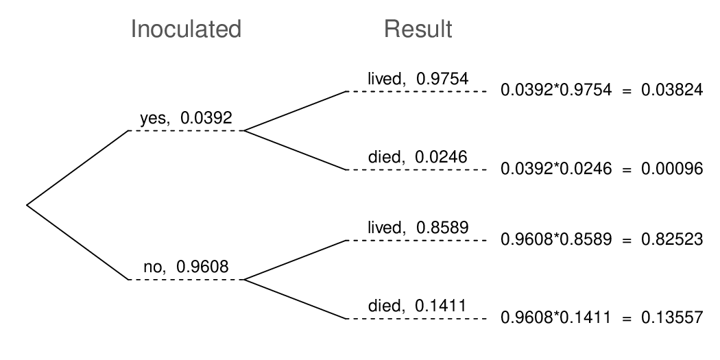
smallpox data set.Tree diagrams are annotated with marginal and conditional probabilities, as shown in Figure 3.2.32. This tree diagram splits the smallpox data by inoculation into the yes and no groups with respective marginal probabilities 0.0392 and 0.9608. The secondary branches are conditioned on the first, so we assign conditional probabilities to these branches. For example, the top branch in Figure 3.2.32 is the probability that lived conditioned on the information that inoculated.
We may (and usually do) construct joint probabilities at the end of each branch in our tree by multiplying the numbers we come across as we move from left to right. These joint probabilities are computed using the General Multiplication Rule:
Example 3.2.33.
What is the probability that a randomly selected person who was inoculated died?
This is equivalent to \(P(\text{died } | \text{ inoculated} )\text{.}\) This conditional probability can be found in the second branch as 0.0246.
Example 3.2.34.
What is the probability that a randomly selected person lived?
There are two ways that a person could have lived: be inoculated and live OR not be inoculated and live. To find this probability, we sum the two disjoint probabilities:
Checkpoint 3.2.35.
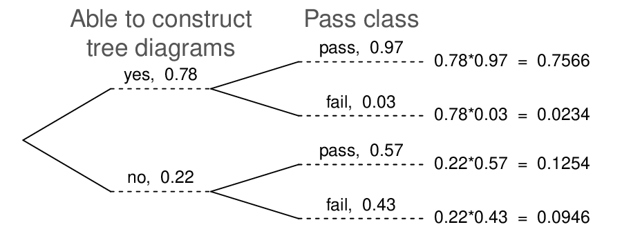
After an introductory statistics course, 78% of students can successfully construct tree diagrams. Of those who can construct tree diagrams, 97% passed, while only 57% of those students who could not construct tree diagrams passed. (a) Organize this information into a tree diagram. (b) What is the probability that a student who was able to construct tree diagrams did not pass? (c) What is the probability that a randomly selected student was able to successfully construct tree diagrams and passed? (d) What is the probability that a randomly selected student passed? 18
(a) The tree diagram is shown to the right.
(b) \(P(\text{not pass } | \text{ able to construct tree diagram}) = 0.03\text{.}\)
(c) \(P(\text{able to construct tree diagrams and passed}) = P(\text{able to construct tree diagrams}) \times P(\text{passed } | \text{ able to construct tree diagrams}) = 0.78 \times 0.97 = 0.7566\text{.}\)
(d) \(P(\text{passed}) = 0.7566 + 0.1254 = 0.8820\text{.}\)
Subsection 3.2.11 Bayes' Theorem
¶In many instances, we are given a conditional probability of the form
but we would really like to know the inverted conditional probability:
For example, instead of wanting to know \(P(\)lived \(|\) inoculated\()\text{,}\) we might want to know \(P(\)inoculated \(|\) lived\()\text{.}\) This is more challenging because it cannot be read directly from the tree diagram. In these instances we use Bayes' Theorem. Let's begin by looking at a new example.
Example 3.2.36.
In Canada, about 0.35% of women over 40 will develop breast cancer in any given year. A common screening test for cancer is the mammogram, but this test is not perfect. In about 11% of patients with breast cancer, the test gives a false negative: it indicates a woman does not have breast cancer when she does have breast cancer. Similarly, the test gives a false positive in 7% of patients who do not have breast cancer: it indicates these patients have breast cancer when they actually do not.If we tested a random woman over 40 for breast cancer using a mammogram and the test came back positive — that is, the test suggested the patient has cancer — what is the probability that the patient actually has breast cancer?
We are given sufficient information to quickly compute the probability of testing positive if a woman has breast cancer (\(1.00 - 0.11 = 0.89\)). However, we seek the inverted probability of cancer given a positive test result:
Here, “has BC” is an abbreviation for the patient actually having breast cancer, and “mammogram\(^+\)” means the mammogram screening was positive, which in this case means the test suggests the patient has breast cancer. (Watch out for the non-intuitive medical language: a positive test result suggests the possible presence of cancer in a mammogram screening.) We can use the conditional probability formula from the previous section: \(P(A|B) = \frac{P(A \text{ and } B)}{P(B)}\text{.}\) Our conditional probability can be found as follows:
The probability that a mammogram is positive is as follows.
A tree diagram is useful for identifying each probability and is shown in Figure 3.2.37. Using the tree diagram, we find that
That is, even if a patient has a positive mammogram screening, there is still only a 4% chance that she has breast cancer.

Example 3.2.36 highlights why doctors often run more tests regardless of a first positive test result. When a medical condition is rare, a single positive test isn't generally definitive.
Consider again the last equation of Example 3.2.36. Using the tree diagram, we can see that the numerator (the top of the fraction) is equal to the following product:
The denominator — the probability the screening was positive — is equal to the sum of probabilities for each positive screening scenario:
In the example, each of the probabilities on the right side was broken down into a product of a conditional probability and marginal probability using the tree diagram.
We can see an application of Bayes' Theorem by substituting the resulting probability expressions into the numerator and denominator of the original conditional probability.
Bayes' Theorem: inverting probabilities.
Consider the following conditional probability for variable 1 and variable 2:
Bayes' Theorem states that this conditional probability can be identified as the following fraction:
where \(A_2\text{,}\) \(A_3\text{,}\) ..., and \(A_k\) represent all other possible outcomes of the first variable.
Bayes' Theorem is just a generalization of what we have done using tree diagrams. The formula need not be memorized, since it can always be derived using a tree diagram:
The numerator identifies the probability of getting both \(A_1\) and \(B\text{.}\)
The denominator is the overall probability of getting \(B\text{.}\) Traverse each branch of the tree diagram that ends with event \(B\text{.}\) Add up the required products.
Example 3.2.38.
Jose visits campus every Thursday evening. However, some days the parking garage is full, often due to college events. There are academic events on 35% of evenings, sporting events on 20% of evenings, and no events on 45% of evenings. When there is an academic event, the garage fills up about 25% of the time, and it fills up 70% of evenings with sporting events. On evenings when there are no events, it only fills up about 5% of the time. If Jose comes to campus and finds the garage full, what is the probability that there is a sporting event? Use a tree diagram to solve this problem.
The tree diagram, with three primary branches, is shown below
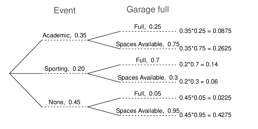
We want:
If the garage is full, there is a 56% probability that there is a sporting event.
The last several exercises offered a way to update our belief about whether there is a sporting event, academic event, or no event going on at the school based on the information that the parking lot was full. This strategy of updating beliefs using Bayes' Theorem is actually the foundation of an entire section of statistics called Bayesian statistics. While Bayesian statistics is very important and useful, we will not have time to cover it in this book.
Subsection 3.2.12 Section summary
A conditional probability can be written as \(P(A | B)\) and is read, “Probability of \(A\) given \(B\)”. \(P(A|B)\) is the probability of \(A\text{,}\) given that \(B\) has occurred. In a conditional probability, we are given some information. In an unconditional probability, such as \(P(A)\text{,}\) we are not given any information.
Sometimes \(P(A | B)\) can be deduced. For example, when drawing without replacement from a deck of cards, \(P(\text{ 2nd draw is an Ace } | \text{ 1st draw was an Ace } ) = \frac{3}{51}\text{.}\) When this is not the case, as when working with a table or a Venn diagram, one must use the conditional probability rule \(P(A | B) = \frac{P(A\text{ and } B)}{P(B)}\text{.}\)
In the last section, we saw that two events are independent when the outcome of one has no effect on the outcome of the other. When \(A\) and \(B\) are independent, \(P(A | B) = P(A)\text{.}\)
When \(A\) and \(B\) are dependent, find the probability of \(A\) and \(B\) using the General Multiplication Rule: \(P(A \text{ and } B) = P(A | B)\times P(B)\text{.}\)
In the special case where \(A\) and \(B\) are independent, \(P(A \text{ and } B) = P(A)\times P(B)\text{.}\)
If \(A\) and \(B\) are mutually exclusive, they must be dependent, since the occurrence of one of them changes the probability that the other occurs to 0.
When sampling without replacement, such as drawing cards from a deck, make sure to use conditional probabilities when solving and problems.
Sometimes, the conditional probability \(P(B|A)\) may be known, but we are interested in the “inverted” probability \(P(A|B)\text{.}\) Bayes' Theorem helps us solve such conditional probabilities that cannot be easily answered. However, rather than memorize Bayes' Theorem, one can generally draw a tree diagram and apply the conditional probability rule \(P(A | B)=\frac{P(A\text{ and } B)}{P(B)}\text{.}\) The resulting answer often has the form \(\frac{w\times x\text{ } +\text{ } y\times z}{w\times x}\text{,}\) where \(w, x, y, z\) are numbers from a tree diagram.
Exercises 3.2.13 Exercises
1. Joint and conditional probabilities.
\(P(A) = 0.3\text{,}\) \(P(B) = 0.7\)
Can you compute \(P(A \text{ and } B)\) if you only know \(P(A)\) and \(P(B)\text{?}\)
-
Assuming that events \(A\) and \(B\) arise from independent random processes,
what is \(P(A \text{ and } B)\text{?}\)
what is \(P(A \text{ or } B)\text{?}\)
what is \(P(A|B)\text{?}\)
If we are given that \(P(A \text{ and } B) = 0.1\text{,}\) are the random variables giving rise to events \(A\) and \(B\) independent?
If we are given that \(P(A \text{ and } B) = 0.1\text{,}\) what is \(P(A|B)\text{?}\)
(a) No, but we could if A and B are independent.
(b-i) 0.21.
(b-ii) 0.79.
(b-iii) 0.3.
(c) No, because 0.1 6= 0.21, where 0.21 was the value computed under independence from part (a).
(d) 0.143.
2. PB & J.
Suppose 80% of people like peanut butter, 89% like jelly, and 78% like both. Given that a randomly sampled person likes peanut butter, what's the probability that he also likes jelly?
3. Global warming.
(VIDEO) A Pew Research poll asked 1,306 Americans “From what you've read and heard, is there solid evidence that the average temperature on earth has been getting warmer over the past few decades, or not?”. The table below shows the distribution of responses by party and ideology, where the counts have been replaced with relative frequencies. 19
| Response | |||||
| Earth is warming |
Not warming |
Don't Know Refuse |
Total | ||
| Party and | Conservative Republican | 0.11 | 0.20 | 0.02 | 0.33 |
| Ideology | Mod/Lib Republican | 0.06 | 0.06 | 0.01 | 0.13 |
| Mod/Cons Democrat | 0.25 | 0.07 | 0.02 | 0.34 | |
| Liberal Democrat | 0.18 | 0.01 | 0.01 | 0.20 | |
| Total | 0.60 | 0.34 | 0.06 | 1.00 | |
Are believing that the earth is warming and being a liberal Democrat mutually exclusive?
What is the probability that a randomly chosen respondent believes the earth is warming or is a liberal Democrat?
What is the probability that a randomly chosen respondent believes the earth is warming given that he is a liberal Democrat?
What is the probability that a randomly chosen respondent believes the earth is warming given that he is a conservative Republican?
Does it appear that whether or not a respondent believes the earth is warming is independent of their party and ideology? Explain your reasoning.
What is the probability that a randomly chosen respondent is a moderate/liberal Republican given that he does not believe that the earth is warming?
(a) No, 0.18 of respondents fall into this combination.
(b) \(0.60+0.20-0.18 = 0.62\text{.}\)
(c) \(0.18/0.20 = 0.9\text{.}\)
(d) \(0.11 / 0.33 \approx 0.33\text{.}\)
(e) No, otherwise the answers to (c) and (d) would be the same.
(f) \(0.06/0.34 \approx 0.18\text{.}\)
4. Health coverage, relative frequencies.
The Behavioral Risk Factor Surveillance System (BRFSS) is an annual telephone survey designed to identify risk factors in the adult population and report emerging health trends. The following table displays the distribution of health status of respondents to this survey (excellent, very good, good, fair, poor) and whether or not they have health insurance.
| Health Status | |||||||
| Excellent | Very good | Good | Fair | Poor | Total | ||
| Health | No | 0.0230 | 0.0364 | 0.0427 | 0.0192 | 0.0050 | 0.1262 |
| Coverage | Yes | 0.2099 | 0.3123 | 0.2410 | 0.0817 | 0.0289 | 0.8738 |
| Total | 0.2329 | 0.3486 | 0.2838 | 0.1009 | 0.0338 | 1.0000 | |
Are being in excellent health and having health coverage mutually exclusive?
What is the probability that a randomly chosen individual has excellent health?
What is the probability that a randomly chosen individual has excellent health given that he has health coverage?
What is the probability that a randomly chosen individual has excellent health given that he doesn't have health coverage?
Do having excellent health and having health coverage appear to be independent?
5. Burger preferences.
A 2010 SurveyUSA poll asked 500 Los Angeles residents, “What is the best hamburger place in Southern California? Five Guys Burgers? In-N-Out Burger? Fat Burger? Tommy's Hamburgers? Umami Burger? Or somewhere else?” The distribution of responses by gender is shown below. 20
| Gender | ||||
| Male | Female | Total | ||
| Best hamburger | Five Guys Burgers | 5 | 6 | 11 |
| place | In-N-Out Burger | 162 | 181 | 343 |
| Fat Burger | 10 | 12 | 22 | |
| Tommy's Hamburgers | 27 | 27 | 54 | |
| Umami Burger | 5 | 1 | 6 | |
| Other | 26 | 20 | 46 | |
| Not Sure | 13 | 5 | 18 | |
| Total | 248 | 252 | 500 | |
Are being female and liking Five Guys Burgers mutually exclusive?
What is the probability that a randomly chosen male likes In-N-Out the best?
What is the probability that a randomly chosen female likes In-N-Out the best?
What is the probability that a man and a woman who are dating both like In-N-Out the best? Note any assumption you make and evaluate whether you think that assumption is reasonable.
What is the probability that a randomly chosen person likes Umami best or that person is female?
(a) No. There are 6 females who like Five Guys Burgers.
(b) \(162/248 = 0.65\text{.}\)
(c) \(181/252 = 0.72\text{.}\)
(d) Under the assumption of a dating choices being independent of hamburger preference, which on the surface seems reasonable: \(0.65 \times 0.72 = 0.468\text{.}\)
(e) \((252 + 6 - 1)/500 = 0.514\text{.}\)
6. Assortative mating.
Assortative mating is a nonrandom mating pattern where individuals with similar genotypes and/or phenotypes mate with one another more frequently than what would be expected under a random mating pattern. Researchers studying this topic collected data on eye colors of 204 Scandinavian men and their female partners. The table below summarizes the results. For simplicity, we only include heterosexual relationships in this exercise. 21
| Partner (female) | |||||
| Blue | Brown | Green | Total | ||
| Self (male) | Blue | 78 | 23 | 13 | 114 |
| Brown | 19 | 23 | 12 | 54 | |
| Green | 11 | 9 | 16 | 36 | |
| Total | 108 | 55 | 41 | 204 | |
What is the probability that a randomly chosen male respondent or his partner has blue eyes?
What is the probability that a randomly chosen male respondent with blue eyes has a partner with blue eyes?
What is the probability that a randomly chosen male respondent with brown eyes has a partner with blue eyes? What about the probability of a randomly chosen male respondent with green eyes having a partner with blue eyes?
Does it appear that the eye colors of male respondents and their partners are independent? Explain your reasoning.
7. Marbles in an urn.
Imagine you have an urn containing 5 red, 3 blue, and 2 orange marbles in it.
What is the probability that the first marble you draw is blue?
Suppose you drew a blue marble in the first draw. If drawing with replacement, what is the probability of drawing a blue marble in the second draw?
Suppose you instead drew an orange marble in the first draw. If drawing with replacement, what is the probability of drawing a blue marble in the second draw?
If drawing with replacement, what is the probability of drawing two blue marbles in a row?
When drawing with replacement, are the draws independent? Explain.
(a) 0.3.
(b) 0.3.
(c) 0.3.
(d) \(0.3 \times 0.3 = 0.09\text{.}\)
(e) Yes, the population that is being sampled from is identical in each draw.
8. Socks in a drawer.
In your sock drawer you have 4 blue, 5 gray, and 3 black socks. Half asleep one morning you grab 2 socks at random and put them on. Find the probability you end up wearing
2 blue socks
no gray socks
at least 1 black sock
a green sock
matching socks
9. Chips in a bag.
Imagine you have a bag containing 5 red, 3 blue, and 2 orange chips.
Suppose you draw a chip and it is blue. If drawing without replacement, what is the probability the next is also blue?
Suppose you draw a chip and it is orange, and then you draw a second chip without replacement. What is the probability this second chip is blue?
If drawing without replacement, what is the probability of drawing two blue chips in a row?
When drawing without replacement, are the draws independent? Explain.
(a) \(2/9\text{.}\)
(b) \(3/9 = 1/3\text{.}\)
(c) \((3/10) \times (2/9) \approx 0.067\text{.}\)
(d) No. In this small population of marbles, removing one marble meaningfully changes the probability of what might be drawn next.
10. Books on a bookshelf.
The table below shows the distribution of books on a bookcase based on whether they are nonfiction or fiction and hardcover or paperback.
| Format | ||||
| Hardcover | Paperback | Total | ||
| Type | Fiction | 13 | 59 | 72 |
| Nonfiction | 15 | 8 | 23 | |
| Total | 28 | 67 | 95 | |
Find the probability of drawing a hardcover book first then a paperback fiction book second when drawing without replacement.
Determine the probability of drawing a fiction book first and then a hardcover book second, when drawing without replacement.
Calculate the probability of the scenario in part (b), except this time complete the calculations under the scenario where the first book is placed back on the bookcase before randomly drawing the second book.
The final answers to parts (b) and (c) are very similar. Explain why this is the case.
11. Student outfits.
In a classroom with 24 students, 7 students are wearing jeans, 4 are wearing shorts, 8 are wearing skirts, and the rest are wearing leggings. If we randomly select 3 students without replacement, what is the probability that one of the selected students is wearing leggings and the other two are wearing jeans? Note that these are mutually exclusive clothing options.
For 1 leggings (L) and 2 jeans (J), there are three possible orderings: LJJ, JLJ, and JJL. The probability for LJJ is \((5/24) \times (7/23) \times (6/22) = 0.0173\text{.}\) The other two orderings have the same probability, and these three possible orderings are disjoint events. Final answer: 0.0519.
12. The birthday problem.
Suppose we pick three people at random. For each of the following questions, ignore the special case where someone might be born on February 29th, and assume that births are evenly distributed throughout the year.
What is the probability that the first two people share a birthday?
What is the probability that at least two people share a birthday?
13. Drawing box plots.
After an introductory statistics course, 80% of students can successfully construct box plots. Of those who can construct box plots, 86% passed, while only 65% of those students who could not construct box plots passed.
Construct a tree diagram of this scenario.
Calculate the probability that a student is able to construct a box plot if it is known that he passed.
(a)
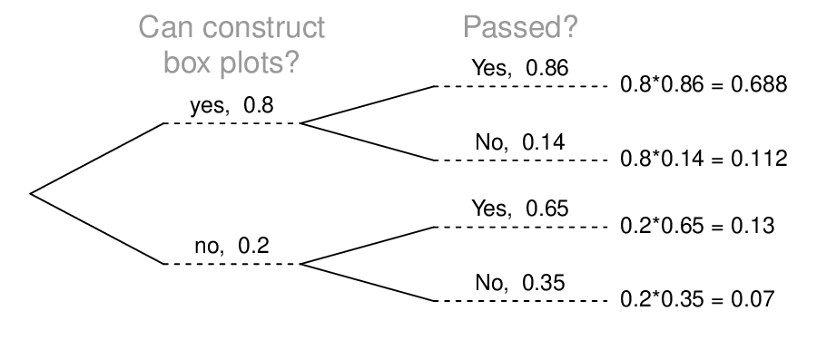
(b) 0.84
14. Predisposition for thrombosis.
A genetic test is used to determine if people have a predisposition for thrombosis, which is the formation of a blood clot inside a blood vessel that obstructs the flow of blood through the circulatory system. It is believed that 3% of people actually have this predisposition. The genetic test is 99% accurate if a person actually has the predisposition, meaning that the probability of a positive test result when a person actually has the predisposition is 0.99. The test is 98% accurate if a person does not have the predisposition. What is the probability that a randomly selected person who tests positive for the predisposition by the test actually has the predisposition?
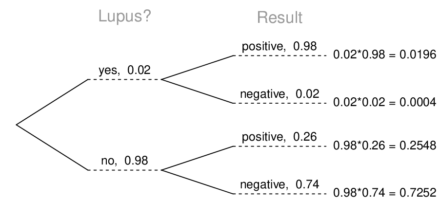
15. It's never lupus.
Lupus is a medical phenomenon where antibodies that are supposed to attack foreign cells to prevent infections instead see plasma proteins as foreign bodies, leading to a high risk of blood clotting. It is believed tha t 2% of the population suffer from this disease. The test is 98% accurate if a person actually has the disease. The test is 74% accurate if a person does not have the disease. There is a line from the Fox television show House that is often used after a patient tests positive for lupus: “It's never lupus.”s Do you think there is truth to this statement? Use appropriate probabilities to support your answer.
0.0714. Even when a patient tests positive for lupus, there is only a 7.14% chance that he actually has lupus. House may be right.
16. Exit poll.
Edison Research gathered exit poll results from several sources for the Wisconsin recall election of Scott Walker. They found that 53% of the respondents voted in favor of Scott Walker. Additionally, they estimated that of those who did vote in favor for Scott Walker, 37% had a college degree, while 44% of those who voted against Scott Walker had a college degree. Suppose we randomly sampled a person who participated in the exit poll and found that he had a college degree. What is the probability that he voted in favor of Scott Walker? 22