Section 26 Atomic Objects
Some PreTeXt objects are relatively indivisable and are used as components of other structures. We call them atomic, even if the term is not perfect. A good example is <image> (next, 26.1). This section is arranged according to these objects and tests the various ways they can be employed.
We frequently include some nonsense text inside short intervening paragraphs to test spacing and establish margins.
Subsection 26.1 <image>
An <image> can be placed in five different ways:
all by itself, as a peer of
<p>typically, with layout control,inside a
<figure>, earning a number and caption,inside a
<sidebyside>, with size and layout configured,inside a
<figure>inside a<sidebyside>, with size and layout configured, with a number and caption, andinside a
<figure>inside a<sidebyside>inside a<figure>, with size and layout configured, with a number and caption, but now sub-numbered ((a), (b), (c),…).
Examples of each, and more.
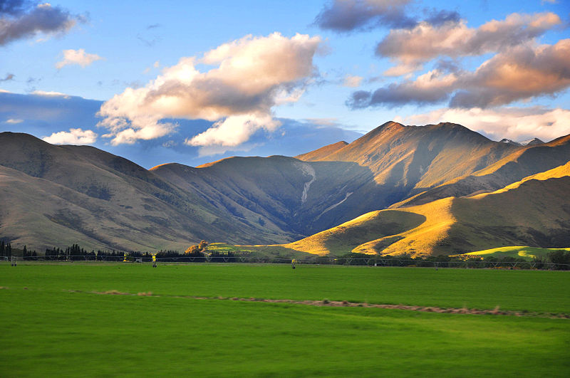
All by itsef, with no layout specified, so showing the default size and placement. Vivamus in congue massa. Morbi condimentum ac magna at accumsan. Vestibulum ac augue eu lorem semper gravida.
Width set at 40%, so equal margins and thus centered. Aenean faucibus augue tellus, et sollicitudin tortor finibus non. Maecenas semper dolor quis diam placerat, iaculis sollicitudin augue finibus. Vestibulum facilisis ligula lectus, ac tristique nisl aliquet non.
Asymmetric margins of 20% and 40% given, implying 40% width, equal to previous instance. Vivamus suscipit diam eget mi cursus viverra.
As a plain component of a <sidebyside>. Widths here are 20% and 30%, margins and gaps are automatic, default alignment on top edges. Nulla pharetra imperdiet elit, in sodales nibh blandit ultricies. Maecenas efficitur ac felis ut pharetra.
Inside a <figure> with no adjustments, so default behavior. Note how a <figure> occupies the entire width of the page, so then does the caption.
Inside a <figure> with asymmetric (large) margins of 30% and 60%. Quisque finibus augue sit amet facilisis fringilla. Aenean faucibus augue tellus, et sollicitudin tortor finibus non.
Inside figures inside a <sidebyside>. Same widths as previous <sidebyside> but alignment on bottoms of the panels, to partially align captions. Note how the captions are constrained in width by the width of the panels of the side-by-side.
Identical code to previous example, but now wrapped in an overall <figure>, which has its own caption and number, leaving the interior figures to be sub-numbered. Cross-references use the full number: Figure 26.5.(b).
Subsection 26.2 <video>
An <video> can be placed in five different ways:
all by itself, as a peer of
<p>typically, with layout control,inside a
<figure>, earning a number and caption,inside a
<sidebyside>, with size and layout configured,inside a
<figure>inside a<sidebyside>, with size and layout configured, with a number and caption, andinside a
<figure>inside a<sidebyside>inside a<figure>, with size and layout configured, with a number and caption, but now sub-numbered ((a), (b), (c),…).
Examples of each, and more.
Videos can be realized in many forms, and can come from a variety of sources. See Section 17 for tests of some of that variety. Here we are testing placement within surroundings and testing the schema for location. But we do have two videos in each test, one provided as a local file and one embedded from a service.
All by itsef, with no layout specified, so showing the default size and placement. Vivamus in congue massa. Morbi condimentum ac magna at accumsan. Vestibulum ac augue eu lorem semper gravida.
Vestibulum facilisis ligula lectus, ac tristique nisl aliquet non. Quisque ornare felis arcu. Vivamus suscipit diam eget mi cursus viverra.
Width set at 40%, so equal margins and thus centered. Aenean faucibus augue tellus, et sollicitudin tortor finibus non. Maecenas semper dolor quis diam placerat, iaculis sollicitudin augue finibus. Vestibulum facilisis ligula lectus, ac tristique nisl aliquet non.
Vestibulum facilisis ligula lectus, ac tristique nisl aliquet non. Quisque ornare felis arcu. Vivamus suscipit diam eget mi cursus viverra.
Asymmetric margins of 20% and 40% given, implying 40% width, equal to previous instance. Vivamus suscipit diam eget mi cursus viverra.
Vestibulum facilisis ligula lectus, ac tristique nisl aliquet non. Quisque ornare felis arcu. Vivamus suscipit diam eget mi cursus viverra.
As a plain component of a <sidebyside>. Widths here are 20% and 30%, margins and gaps are automatic, default alignment on top edges. Nulla pharetra imperdiet elit, in sodales nibh blandit ultricies. Maecenas efficitur ac felis ut pharetra.
Inside a <figure> with no adjustments, so default behavior. Note how a <figure> occupies the entire width of the page, so then does the caption.
Vestibulum facilisis ligula lectus, ac tristique nisl aliquet non. Quisque ornare felis arcu. Vivamus suscipit diam eget mi cursus viverra.
Inside a <figure> with asymmetric (large) margins of 30% and 60%. Quisque finibus augue sit amet facilisis fringilla. Aenean faucibus augue tellus, et sollicitudin tortor finibus non.
Vestibulum facilisis ligula lectus, ac tristique nisl aliquet non. Quisque ornare felis arcu. Vivamus suscipit diam eget mi cursus viverra.
Inside figures inside a <sidebyside>. Same widths as previous <sidebyside> but alignment on bottoms of the panels, to partially align captions. Note how the captions are constrained in width by the width of the panels of the side-by-side.
Identical code to previous example, but now wrapped in an overall <figure>, which has its own caption and number, leaving the interior figures to be sub-numbered. Cross-references use the full number: Figure 26.12.(b).
Subsection 26.3 <program>, <console>
A <program> and/or <console> can be placed in at least six different ways:
all by itself, as a peer of
<p>typically, with layout controlinside a
<listing>, earning a number and caption, with layout controlinside a
<sidebyside>, with size and layout configuredinside a
<sidebyside>, with size and layout configured, and inside a<figure>inside a
<sidebyside>, with size and layout configured, with each inside a<listing>, earning different numbersinside a
<figure>inside a<sidebyside>inside a<listing>, with size and layout configured, with a number and caption, but now sub-numbered ((a), (b), (c),…).
Examples of each, and more.
Programs can be realized in many forms, and can come from a variety of sources. See Section 17 for tests of some of that variety. Here we are testing placement within surroundings and testing the schema for location. But we do have two videos in each test, one provided as a local file and one embedded from a service.
All by itsef, with no layout specified, so showing the default size and placement. Vivamus in congue massa. Morbi condimentum ac magna at accumsan. Vestibulum ac augue eu lorem semper gravida.
n_loops <- 10
x.means <- numeric(n_loops)  # create a vector of zeros for results
for (i in 1:n_loops){
    x <- as.integer(runif(100, 1, 7))  # 1 to 6, uniformly
    x.means[i] <- mean(x)
}
x.means
Now a program with shorter lines, with no layout control.
/* Hello World program */

#include<stdio.h>

main()
{
    printf("Hello, World!");
}
And a <console> element, also with no layout control.
pi@raspberrypi ~/progs/chap02 $ gcc -o intAndFloat intAndFloat.c
pi@raspberrypi ~/progs/chap02 $ ./intAndFloat
The integer is 19088743 and the float is 19088.742188
pi@raspberrypi ~/progs/chap02 $
Now similar examples, but with layout control: margins and width.
A <program> with a @width attribute, so centered and with equal margins. Note how the lines word wrap due to the smaller width.
n_loops <- 10
x.means <- numeric(n_loops)  # create a vector of zeros for results
for (i in 1:n_loops){
    x <- as.integer(runif(100, 1, 7))  # 1 to 6, uniformly
    x.means[i] <- mean(x)
}
x.means
A <program> with short lines, so significant, and asymmetric margins, which experimentally do not induce any word-wrapping.
/* Hello World program */

#include<stdio.h>

main()
{
    printf("Hello, World!");
}
A longer <console>, with margins so significant the appearance is ill-advised.
pi@raspberrypi ~/progs/chap02 $ gcc -Wall -o intAndFloat intAndFloat.c
pi@raspberrypi ~/progs/chap02 $ ./intAndFloat
The integer is 19088743 and the float is 19088.742188
pi@raspberrypi ~/progs/chap02 $
Two <listing>, with <caption>, and no layout control.
/* Hello World program */

#include<stdio.h>

main()
{
    printf("Hello, World!");
}
pi@raspberrypi ~/progs/chap02 $ gcc -Wall -o intAndFloat intAndFloat.c
pi@raspberrypi ~/progs/chap02 $ ./intAndFloat
The integer is 19088743 and the float is 19088.742188
pi@raspberrypi ~/progs/chap02 $
Same two <listing>, but now with layout control on the <program> and <console>.
/* Hello World program */

#include<stdio.h>

main()
{
    printf("Hello, World!");
}
pi@raspberrypi ~/progs/chap02 $ gcc -Wall -o intAndFloat intAndFloat.c
pi@raspberrypi ~/progs/chap02 $ ./intAndFloat
The integer is 19088743 and the float is 19088.742188
pi@raspberrypi ~/progs/chap02 $
This <sidebyside> gives each panel a 30% width. The remaining 10% is apportioned for margins and separation.
/* Hello World program */

#include<stdio.h>

main()
{
    printf("Hello, World!");
}
pi@raspberrypi ~/progs/chap02 $ gcc -Wall -o intAndFloat intAndFloat.c
pi@raspberrypi ~/progs/chap02 $ ./intAndFloat
The integer is 19088743 and the float is 19088.742188
pi@raspberrypi ~/progs/chap02 $
n_loops <- 10
x.means <- numeric(n_loops)  # create a vector of zeros for results
for (i in 1:n_loops){
    x <- as.integer(runif(100, 1, 7))  # 1 to 6, uniformly
    x.means[i] <- mean(x)
}
x.means
This is the same three-panel <sidebyside>, but now inside of a <figure>, earning a number and a <caption>.
/* Hello World program */

#include<stdio.h>

main()
{
    printf("Hello, World!");
}
pi@raspberrypi ~/progs/chap02 $ gcc -Wall -o intAndFloat intAndFloat.c
pi@raspberrypi ~/progs/chap02 $ ./intAndFloat
The integer is 19088743 and the float is 19088.742188
pi@raspberrypi ~/progs/chap02 $
n_loops <- 10
x.means <- numeric(n_loops)  # create a vector of zeros for results
for (i in 1:n_loops){
    x <- as.integer(runif(100, 1, 7))  # 1 to 6, uniformly
    x.means[i] <- mean(x)
}
x.means
Finally, a smaller <program> and a smaller <console>, each inside a <listing>, as the two panels of a <sidebyside> with no margins, and slightly different widths (to control word-wrapping). The panels have been aligned vertically so their captions align.
/* Hello World program */

#include<stdio.h>

main()
{
    printf("Hello, World!");
}
$ gcc -Wall -o intAndFloat intAndFloat.c
$ ./intAndFloat
The integer is 19088743 and the float is 19088.742188
$
And again, the two-panel <sidebyside> of <listing>, but now inside a <figure> that has a number and a caption. And then the <listing> are sub-numbered as (a) and (b).
/* Hello World program */

#include<stdio.h>

main()
{
    printf("Hello, World!");
}
$ gcc -Wall -o intAndFloat intAndFloat.c
$ ./intAndFloat
The integer is 19088743 and the float is 19088.742188
$
Subsection 26.4 <tabular>
A <tabular> can be placed in six different ways:
all by itself, as a peer of
<p>typically, with no layout control and hence with a “natural width,” and centeredall by itself, as a peer of
<p>typically, with explicit layout control,inside a
<table>, earning a number and title,inside a
<sidebyside>, with size and layout configured,inside a
<table>inside a<sidebyside>, with size and layout configured, with a number and title, andinside a
<table>inside a<sidebyside>inside a<figure>, with size and layout configured, with a number and title, but now sub-numbered ((a), (b), (c),…).
Examples of each, and more.
A <tabular> realized by LaTeX will normally be as wide as necessary to hold the content, without word-wrapping the content of any cell that is not explicitly authored that way. So for PreTeXt output as LaTeX, when you explicitly constrain the width (including use as a panel of a <sidebyside>, or even setting margins) the table will be scaled, which can result in an apparent font size very different than the surrounding document. [NOT SURE HOW HTML WILL BEHAVE]
Data in a table form can be placed in amongst a series of paragraphs. With no layout control, it will occupy its “natural width” and be centered.
| State | Population | Area (sq. mi.) | Statehood (Year) |
|---|---|---|---|
| Washington | 7,614,893 | 71,362 | 1889 |
| Oregon | 4,217,737 | 98,381 | 1859 |
| California | 39,512,223 | 163,696 | 1850 |
The same effect can be had by specifying that the @width attribute have the value auto, but do not specify any @margins. We test multiple footnotes in a <tabular>, not included in a <table>.
| State 1 | Population | Area (sq. mi.) | Statehood (Year) |
|---|---|---|---|
| Washington | 7,614,893 | 71,362 | 1889 |
| Oregon | 4,217,737 | 98,381 | 1859 |
| California | 39,512,223 2 | 163,696 | 1850 |
In amongst a run of paragraphs (or similar) a <tabular> can be placed with layout control. For LaTeX output, this will scale the table to fit within the explicit, or implicit, width. This can result in obvious differences in the apparent font size. We first have a @width that is experimentally similar to the natural width, with asymetric margins. Then a narrow width, and a wide width, as an illustration.
| State | Population | Area (sq. mi.) | Statehood (Year) |
|---|---|---|---|
| Washington | 7,614,893 | 71,362 | 1889 |
| Oregon | 4,217,737 | 98,381 | 1859 |
| California | 39,512,223 | 163,696 | 1850 |
Narrow. 45% width. 20% margin left, 35% margin right.
| State | Population | Area (sq. mi.) | Statehood (Year) |
|---|---|---|---|
| Washington | 7,614,893 | 71,362 | 1889 |
| Oregon | 4,217,737 | 98,381 | 1859 |
| California | 39,512,223 | 163,696 | 1850 |
Wide. 97% width. 1% margin left, 2% right.
| State | Population | Area (sq. mi.) | Statehood (Year) |
|---|---|---|---|
| Washington | 7,614,893 | 71,362 | 1889 |
| Oregon | 4,217,737 | 98,381 | 1859 |
| California | 39,512,223 | 163,696 | 1850 |
Naturally, a <tabular> can be placed inside a <table>, earning a number and a title.
| State | Population | Area (sq. mi.) | Statehood (Year) |
|---|---|---|---|
| Washington | 7,614,893 | 71,362 | 1889 |
| Oregon | 4,217,737 | 98,381 | 1859 |
| California | 39,512,223 | 163,696 | 1850 |
A little narrower, but still centered by default.
| State | Population | Area (sq. mi.) | Statehood (Year) |
|---|---|---|---|
| Washington | 7,614,893 | 71,362 | 1889 |
| Oregon | 4,217,737 | 98,381 | 1859 |
| California | 39,512,223 | 163,696 | 1850 |
Very narrow, asymmetric margins.
| State | Population | Area (sq. mi.) | Statehood (Year) |
|---|---|---|---|
| Washington | 7,614,893 | 71,362 | 1889 |
| Oregon | 4,217,737 | 98,381 | 1859 |
| California | 39,512,223 | 163,696 | 1850 |
Wider than necessary, asymmetric margins.
| State | Population | Area (sq. mi.) | Statehood (Year) |
|---|---|---|---|
| Washington | 7,614,893 | 71,362 | 1889 |
| Oregon | 4,217,737 | 98,381 | 1859 |
| California | 39,512,223 | 163,696 | 1850 |
Now into <sidebyside> in various ways and with various sizes. First, two <tabular> as panels with widths at 60% and 30%.
| State | Population | Area (sq. mi.) | Statehood (Year) |
|---|---|---|---|
| Washington | 7,614,893 | 71,362 | 1889 |
| Oregon | 4,217,737 | 98,381 | 1859 |
| California | 39,512,223 | 163,696 | 1850 |
| \(x\) | \(f(x)\) |
|---|---|
| 3 | 9.734 |
| 5 | 2.175 |
Let's do that again, but with widths experimentally set to make font sizes match.
| State | Population | Area (sq. mi.) | Statehood (Year) |
|---|---|---|---|
| Washington | 7,614,893 | 71,362 | 1889 |
| Oregon | 4,217,737 | 98,381 | 1859 |
| California | 39,512,223 | 163,696 | 1850 |
| \(x\) | \(f(x)\) |
|---|---|
| 3 | 9.734 |
| 5 | 2.175 |
Same tabular, which fills roughly 80% by itself, packed into a single <sidebyside> with just a 2% gap, and no side margins.
| State | Population | Area (sq. mi.) | Statehood (Year) |
|---|---|---|---|
| Washington | 7,614,893 | 71,362 | 1889 |
| Oregon | 4,217,737 | 98,381 | 1859 |
| California | 39,512,223 | 163,696 | 1850 |
| State | Population | Area (sq. mi.) | Statehood (Year) |
|---|---|---|---|
| Washington | 7,614,893 | 71,362 | 1889 |
| Oregon | 4,217,737 | 98,381 | 1859 |
| California | 39,512,223 | 163,696 | 1850 |
Natural widths, but now as a pair of tables.
| State | Population | Area (sq. mi.) | Statehood (Year) |
|---|---|---|---|
| Washington | 7,614,893 | 71,362 | 1889 |
| Oregon | 4,217,737 | 98,381 | 1859 |
| California | 39,512,223 | 163,696 | 1850 |
| \(x\) | \(f(x)\) |
|---|---|
| 3 | 9.734 |
| 5 | 2.175 |
Finally, as two individual <table>, grouped and laid out via a <sidebyside>, and collected as a <figure>. Which causes sub-numbering of the enclosed <table>.
| State | Population | Area (sq. mi.) | Statehood (Year) |
|---|---|---|---|
| Washington | 7,614,893 | 71,362 | 1889 |
| Oregon | 4,217,737 | 98,381 | 1859 |
| California | 39,512,223 | 163,696 | 1850 |
| \(x\) | \(f(x)\) |
|---|---|
| 3 | 9.734 |
| 5 | 2.175 |